Fabric Lamina Analysis

How the fabric lamina calculator predicts elastic properties of woven composite plies from fiber, matrix, and weave geometry using analytical RVE-based homogenization.

Why Fabric Lamina Analysis?

Aircraft skins, automotive panels, wind turbine blades, sporting goods: woven reinforcement is everywhere. Where unidirectional (UD) tape runs its fibers in one direction only, a woven fabric interlaces yarns in two. That is what gives it drapability and impact resistance, and it is also what makes the properties harder to predict. Every yarn has to travel up over and down under each crossing yarn it meets, and that undulation leaves in-plane stiffness below what the same fibers would give you in a flat UD ply.

Standard Classical Lamination Theory treats every ply as a flat, homogeneous orthotropic layer. For UD plies that holds. A woven ply is not homogeneous: properties change from point to point across the lamina as the yarns rise and fall. So the fabric lamina builder computes one equivalent homogeneous set of constants (E₁, E₂, G₁₂, v₁₂, CTE, CME) for the whole woven ply, and the rest of the CLT pipeline never has to know the ply was woven. The diagram below shows the four levels: constituent properties go through micromechanics to give yarn constants, and those combine with the weave geometry in an RVE-based homogenization step to give the equivalent lamina properties.

This page walks through each level. It stops short of the full derivations: for shape functions, integration procedures, and ABD matrix assembly, see the references at the bottom of this page.

Supported Weave Patterns

The weave pattern determines how many of each basic element type appear in the unit cell. ABD Composites supports five patterns:

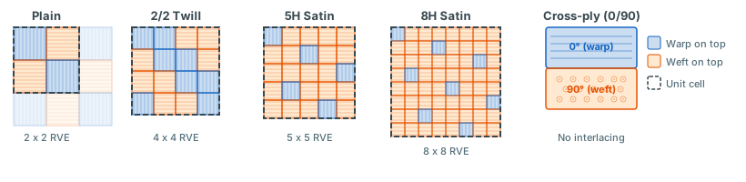
In the diagrams below, blue cells indicate warp on top and orange cells indicate weft on top.

Pattern	Description
	Plain weave: Each warp yarn alternates over and under every weft yarn. Highest crimp (undulation), most balanced. The simplest and most common weave pattern.
	2/2 Twill: Each yarn floats over two and under two crossing yarns, creating a diagonal pattern. Less crimp than plain weave, better drape. Common in automotive and sporting goods.
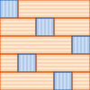	5-Harness Satin: Each yarn floats over four and under one crossing yarn. Low crimp, smoother surface finish. Used in aerospace where surface quality and stiffness matter.
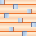	8-Harness Satin: Each yarn floats over seven and under one. Minimal crimp, closest to UD-like stiffness in-plane. Preferred for high-performance aerospace structures.
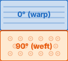	Cross-ply (0/90): Two flat (non-undulating) UD plies stacked at 0 and 90 degrees. No yarn interlacing. Useful as a validation baseline (results should match two UD plies at 0/90 in the laminate builder) or for modelling non-crimp fabrics (NCFs).

Less undulation, higher in-plane stiffness. Plain weave sits at one end with the most undulation, and satin weaves sit at the other, close to the stiffness of the equivalent cross-ply laminate. You pay for that in handling: the long floats of a satin make the fabric less stable and the yarns easier to shift out of place.

Most commercial fabrics are balanced, meaning the warp and weft yarns share the same tow size, spacing, and geometry, which makes E₁ = E₂. The builder has a balanced weave toggle that locks the warp and weft geometry fields together, so you enter one set of values instead of two. Turn it off for unbalanced fabrics, where the tow sizes or yarn counts differ between warp and weft, and enter each direction separately.

RVE-Based Homogenization

The calculation uses a Representative Volume Element (RVE) approach.¹²³ Find the smallest repeating unit cell of the weave, divide it into basic elements, apply CLT pointwise at each integration point, then assemble the results under an iso-strain assumption to get equivalent lamina stiffnesses.

The process follows these steps:

1. Define the unit cell geometry. You specify warp/weft yarn counts (C_x, C_y), yarn widths and heights, layer thickness, and fiber volume fraction. From these, the calculator determines the yarn geometry within the repeating unit cell.
2. Compute yarn properties. Fiber and matrix properties are combined using your chosen micromechanics model to get the yarn-level elastic constants (E₁, E₂, G₁₂, v₁₂) and thermal properties (CTE, CME). The fiber volume fraction in the yarn is derived from the global V_f and yarn geometry.
3. Pointwise CLT integration. The unit cell is divided into four basic element types (A, B, C, D), each representing a different combination of yarn undulation (see below). At each integration point, the local yarn undulation angle is computed from the shape function, and the yarn stiffness matrices are rotated accordingly. A local CLT calculation then produces the full [A], [B], and [D] matrices (extensional, coupling, and bending stiffness) for that point. The integration uses Gauss-Legendre quadrature, a numerical method that evaluates the integral by sampling at optimally chosen points and weighting each sample. With relatively few points it captures the continuously varying yarn undulation across the element.
4. Iso-strain assembly. The element-level ABD matrices are averaged over each basic element, then combined using element counts specific to the weave pattern. The result is a fabric-level set of [A], [B], and [D] matrices representing the entire unit cell. The [B] matrix captures bending-extension coupling that arises in asymmetric weaves such as satin patterns.
5. Extract equivalent properties. The fabric [A] matrix is inverted to get compliance, from which E_xx, E_yy, G_xy, and v_xy are extracted. Equivalent CTE and CME are computed from the thermal and moisture force resultants.

The Four Basic Elements

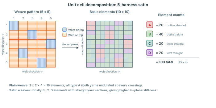
Every weave pattern comes apart into a repeating unit cell (RVE) built from four basic element types (A, B, C, D). How far the RVE subdivides follows the weave. A 5-harness satin RVE, for example, contains 5 x 5 yarn crossings, and each crossing splits into a 2 x 2 grid of basic elements, so 100 elements in total. Each one covers a small region with its own combination of warp and weft yarn shape:

• Element A: Both warp and weft yarns are undulated (crossing point where one yarn passes over the other).
• Element B: Both warp and weft yarns are straight (yarns run flat, not crossing).
• Element C: Warp yarn is straight, weft yarn is undulated.
• Element D: Warp yarn is undulated, weft yarn is straight.

The weave pattern sets how many of each type appear in the unit cell, and which yarn (warp or weft) is on top in each. A plain weave is all A-type elements, because every crossing involves undulation. Satin weaves are mostly B, C, and D types, where at least one yarn runs straight, and that is where their higher in-plane stiffness comes from.

The decomposition also exposes something about satin: it is asymmetric about its own midplane. In a 5-harness satin, one set of yarns spends most of the unit cell on top and the other spends most of it on the bottom. That gives a non-zero [B] coupling matrix inside the unit cell, so the fabric layer on its own has bending-extension coupling. Plain and twill weaves keep equal amounts of warp and weft above and below the midplane, so their [B] matrix is zero.

The builder computes the full ABD matrices internally, but what it reports is equivalent in-plane properties (from the [A] matrix), for every weave type including satin. That matches shop practice: satin layers are flipped alternately during stacking, so the asymmetry of one layer cancels against its neighbour at the laminate level. For that use the in-plane constants are the right answer, and they feed straight into the CLT laminate analysis.

Unit Cell Geometry

The geometry inputs define the shape and packing of yarns within one repeating unit of the weave. These parameters can be measured from micrographs of polished cross-sections, or obtained from fabric supplier datasheets.

• Weft count (C_x) and Warp count (C_y): Number of yarns per millimeter in the weft and warp directions. These counts determine the size of the basic elements: the element width is 1/(2C_x) and the element length is 1/(2C_y).
• Weft yarn width (w_we) and Warp yarn width (w_wa): The width of the flattened yarn cross-section in millimeters. Warp and weft yarns can have different widths, especially in unbalanced fabrics.
• Weft yarn height (h_we) and Warp yarn height (h_wa): The thickness of the yarn cross-section. Together with width, this defines the elliptical yarn shape used in the undulation model.
• Layer thickness (h_lay): The total thickness of a single fabric ply (not the yarn height). Typically larger than the sum of warp and weft yarn heights, because of nesting and resin-rich regions.
• V_f (fiber volume fraction): The global fiber volume fraction of the laminate. The calculator uses this together with the yarn geometry to derive the fiber volume fraction inside the yarn (V_f,yarn), which is what the micromechanics models actually need.

Yarn Geometry Model

Within each basic element, the yarn geometry is described by two components: a cross-sectional shape and an undulation midline.

The yarn cross-section is modelled as an ellipse, defined by the yarn width and height. Warp and weft yarns can have different cross-sections, which matters for unbalanced fabrics where the two yarn directions use different tow sizes or experience different compaction.

The model also carries resin-rich regions, the pure matrix pockets above and below the yarns. Give it a layer thickness h_lay larger than the sum of the warp and weft yarn heights and those matrix-filled gaps go into the stiffness calculation on their own account. They hold no fibers, so they add compliance to the fabric layer.

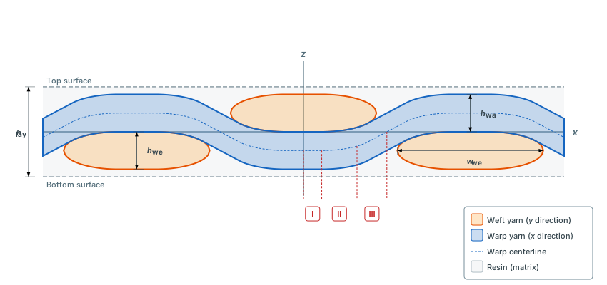
The undulation midline describes the path the yarn centre takes as it passes over and under crossing yarns. The model uses a three-zone function as shown in the diagram below:

• Zone I (flat contact zone): The region where the yarn runs flat while in contact with the crossing yarn beneath it. The length of this zone is controlled by the undulation factor.
• Zone II (elliptical transition zone): An elliptical curve describing the yarn bending away from the contact region as it rises or falls to pass over or under the crossing yarn.
• Zone III (free tangent zone): A straight line tangent to the ellipse, connecting the end of the undulation curve to the edge of the basic element where it meets the next crossing.

Three zones beat a pure sinusoid here, because a real yarn flattens where it presses against its neighbour instead of curving through the contact. The shape is set by the undulation factors (U_x and U_y for the weft and warp directions), defined as U = 1 - (flat length)/(total yarn width). At 1.0 there is no flat contact zone at all and the yarn follows a pure elliptical path; at 0.0 the yarn is straight. Both are inputs in the builder. The weave presets fill them in, and you can override them to match the fabric in front of you.

Fiber volume fraction in the yarn

The micromechanics models need the fiber volume fraction inside the yarn (V_f,yarn), not the global laminate V_f. The calculator derives V_f,yarn by comparing the total volume of the basic element to the volume occupied by the yarns (obtained by integrating the shape functions). Because the yarn volume is always less than the total element volume (the remainder is pure matrix), V_f,yarn is always higher than the global V_f. This is physically correct: fibers are densely packed inside the yarn bundles, with resin-rich regions filling the gaps between yarns. The section below shows this: every fiber lives inside a yarn outline, and the resin-rich regions between yarns hold none.

Because V_f,yarn is derived rather than entered, it is the one quantity on this page that can quietly come out physically impossible. Fibers are circular cylinders, and there is a hard ceiling on how tightly equal circles can be packed into a plane:

• 78.5% (square packing), equal to π/4. Fibers sitting on a square grid, each touching four neighbours. Above this figure the fibers can no longer be arranged on a square grid at all, so the packing has to be at least partly hexagonal.
• 90.7% (hexagonal close packing), equal to π/(2√3). The densest possible arrangement of equal circles. Nothing can pack tighter than this, in a yarn or anywhere else.

The fiber diameter is identical in all three panels above and only the spacing changes, so past the right-hand one the circles would have to overlap. The builder warns above 78.5% and refuses to calculate above 90.7%. The refusal is deliberate rather than cautious: above the hexagonal limit the geometry you described cannot exist, so the micromechanics models would happily return yarn constants for it and every number downstream would be fiction. Real consolidated tows sit well below both figures, typically 60% to 75%, because even a tightly compacted bundle keeps some resin between the fibers and the fibers are never perfectly ordered. Treat anything above 80% as a sign that the unit cell needs revisiting, not as a high-performance result.

V_f,yarn rises when the yarns you described are too small to hold the fiber content you asked for. Four inputs move it, listed here strongest first:

• Increase the yarn widths and heights. This is the biggest lever by a wide margin, because it directly increases the yarn volume that the fibers are packed into. Widening the yarns of a 102% unit cell from 0.16 mm to 0.19 mm brings it to 85%. Note that yarn width cannot exceed the available spacing set by the yarn counts, which is checked separately.
• Lower the global V_f. V_f,yarn scales linearly with it, so this is the most predictable adjustment. Worth a look first if the V_f you entered came from a datasheet for a different fabric architecture.
• Reduce the layer thickness. A thinner ply at the same yarn cross-section means less resin-rich space in the unit cell, so the same fiber content spreads over proportionally more yarn. The layer thickness must still be at least the sum of the warp and weft yarn heights.
• Lower the undulation factors. A more undulated yarn spends less of the unit cell at its full height, which shrinks the yarn volume and pushes V_f,yarn up. This is the weakest of the four and the one most constrained by the weave pattern you are actually modelling, so change it last.

The V_f,yarn figure itself is reported in the Yarn Properties panel of the builder, so you can watch it move as you adjust the geometry rather than working blind against the validation message.

You do not have to tune these by hand. Each geometry field in the builder has an auto-fill button that derives its value from the fields you have already entered, using the standard relationships between them:

• Yarn width from yarn count: w = 0.9/C, so the yarns fill 90% of the available spacing and leave a realistic gap between neighbours.
• Yarn count from yarn width: C = 1/w, the reverse relationship, assuming yarns that just touch.
• Yarn height from yarn width: h = w/8, a 4:1 flattened aspect ratio split between the warp and weft yarns.
• Layer thickness from yarn heights: h_lay = 1.1 (h_wa + h_we), the minimum that fits both yarns plus 10% for the resin-rich region.

Working down the geometry card and using each auto-fill in turn (width from count, then height from width, then layer thickness from the heights) produces a self-consistent unit cell and is the quickest way out of a packing violation. Applied to the builder's own weave presets it lands V_f,yarn between 61% and 74% for every weave pattern, comfortably inside the realistic range for a consolidated tow. Keep your own measured values wherever you have them, and use the auto-fills for the fields you are guessing at.

Micromechanics Models

The fabric lamina builder uses the same micromechanics models available in the UD lamina builder. They combine fiber and matrix properties at a given volume fraction to predict the yarn-level constants. One thing changes: here the micromechanics runs at the yarn level, on V_f,yarn, not at the laminate level.

The elastic and thermal models are chosen independently for the yarn property calculation. The micromechanics page compares them side by side, with the equations and guidance on which to pick.

What the Builder Outputs

The fabric lamina builder produces two levels of output:

Equivalent lamina properties

The main results: equivalent homogeneous, orthotropic material constants for the fabric ply. Save them as a lamina in your material library and they are available to the laminate builder, structural analysis, and failure analysis like any other material.

• E_x, E_y: Equivalent moduli in the weft (x) and warp (y) directions [GPa].
• G_xy: Equivalent in-plane shear modulus [GPa].
• v_xy: Equivalent Poisson's ratio.
• CTE (α_x, α_y): Equivalent coefficients of thermal expansion in the weft (x) and warp (y) directions [ppm/°C]. Only shown when both fiber and matrix CTE data is provided.
• CME (β_x, β_y): Equivalent coefficients of moisture expansion in the weft (x) and warp (y) directions. Only shown when both fiber and matrix CME data is provided.
• Density, FAW, and TAW: Composite density [g/cm³], fiber areal weight [g/m²], and total areal weight [g/m²], when constituent density data is available. See the ply calculator for how these tie back to fiber volume fraction and cured ply thickness.

Yarn-level properties

Intermediate results showing the micromechanics output at the yarn level: E₁, E₂, G₁₂, v₁₂, and CTE/CME of the impregnated yarn before undulation effects are applied. Handy for checking your inputs, and for seeing how much of the fabric response the yarn itself accounts for.

From Fabric Ply to Laminate

Once you have your equivalent lamina properties, the workflow is the same as for UD plies:

1. Save the lamina to your material library from the fabric builder page.
2. Build a laminate using the laminate builder. Add your fabric lamina as layers with the appropriate angles and thicknesses.
3. Run analysis: the laminate's ABD matrix, engineering constants, first ply failure, and structural analysis all work with fabric laminae the same way they work with UD laminae.

That is the whole point of homogenizing. The internal structure of the woven ply collapses into a handful of constants, and nothing downstream of it has to change.

Assumptions and Limitations

The builder is aimed at preliminary design and material trade studies. What it assumes, and where it stops:

• Elastic properties only. The builder predicts stiffness (moduli, Poisson's ratio, CTE). It does not predict fabric-level strengths. Strength prediction for woven composites requires damage modelling that goes beyond closed-form homogenization.
• Iso-strain (Parallel-Parallel) assembly. The Parallel-Parallel model assumes uniform in-plane strain across all basic elements (upper-bound stiffness estimate), as opposed to the iso-stress or Series-Series model (lower-bound). Lamers¹ found the iso-strain approach to be closer to experimental data than the iso-stress alternative. The model does compute full [B] coupling matrices for asymmetric weaves.
• Idealized yarn geometry. Yarn cross-sections are modelled as ellipses, and undulation paths use a three-zone shape function (flat contact, elliptical transition, straight free section). Real yarn shapes vary with compaction pressure and nesting. This idealized model is standard in the literature¹²³ and gives good agreement with experimental data for typical fabric architectures.
• No yarn-yarn interaction. The model does not account for contact mechanics between crossing yarns. This is acceptable for typical processing conditions but may matter at very high fiber volume fractions.
• Linear elastic. Like all tools in ABD Composites, the analysis assumes linear elastic material behavior. Nonlinear effects (matrix yielding, progressive damage) are not captured.
• Orthogonal weaves only. The current implementation assumes yarns are orthogonal (warp and weft at 90 degrees to each other). Skewed fabric geometries (disalignment angle θ ≠ 0) are not currently supported.

Why an Analytical RVE Model?

There are broadly two families of methods for predicting fabric lamina properties: analytical models (closed-form equations) and finite element (FE) unit cell models.

FE-based methods³ mesh the unit cell geometry and solve the equilibrium equations numerically. That buys you detailed stress distributions inside individual yarns and out-of-plane properties. It also costs you dedicated FE software, minutes to hours per run, and a new mesh for every weave architecture. Nothing about that fits a tool that has to answer while you are still typing.

Analytical RVE models go the other way. They describe the yarn geometry with shape functions, apply CLT at integration points across the unit cell, and average the result. Milliseconds, in a browser tab, and the same parameterization covers every weave pattern by changing the element counts.

So what does the shortcut cost in accuracy? A 2024 comparison study by Lopez-Santos et al.⁴ put the question directly. They compared two analytical micromechanical models (a CLT-based bending-restrained model and a 3D series-parallel model) against a dedicated FE unit cell model for E-glass/vinyl ester plain weave composites, with the geometric inputs measured from micrographs at 100 measurements per parameter. Their findings:

• In-plane properties: both analytical models achieved good agreement with FE predictions and experimental measurements for E_x, E_y, G_xy, and v_xy.
• Out-of-plane properties: only the FE model predicted E_z, G_xz, and G_yz accurately. The analytical models overpredicted these values.
• Input quality matters: every model's accuracy depended strongly on how well the yarn geometry had been characterized. Measured parameters did clearly better than nominal values.

CLT-based laminate analysis uses only in-plane lamina properties, which is what the ABD matrix describes. On those, the analytical RVE approach matches FE closely enough while running in milliseconds instead of minutes. The out-of-plane limitation never comes up in thin laminate analysis.

Independent formulations of the analytical RVE approach have been published since the early 1990s.¹² The ABD Composites implementation handles asymmetric weaves (satin patterns, where warp and weft are not balanced about the midplane) and lets warp and weft yarns take different cross-sections.

Author: Rick Schrijver

References

1. Lamers, E. A. D. (2004). Shape distortions in fabric reinforced composite products due to processing induced fibre reorientation. PhD thesis, University of Twente. URN: urn:nbn:nl:ui:28-41422. Open access
2. Naik, N. K. & Shembekar, P. S. (1992). Elastic behavior of woven fabric composites: I - Lamina analysis. Journal of Composite Materials, 26(15), 2196-2225. doi:10.1177/002199839202601502
3. Lomov, S. V. et al. (2001). Textile composites: modelling strategies. Composites Part A, 32(10), 1379-1394. doi:10.1016/S1359-835X(01)00038-0
4. Lopez-Santos, F. et al. (2024). Prediction of elastic properties of woven polymer composites using micromechanical models and measured microstructural parameters. Journal of Reinforced Plastics and Composites. doi:10.1177/07316844241273025

Frequently Asked Questions