
Composite Micromechanics
How ABD Composites predicts lamina properties from fiber and matrix constituents.
What is Micromechanics?
Micromechanics is the branch of composite mechanics that predicts the bulk engineering properties of a ply (lamina) from the properties of its constituents: fiber and matrix. Instead of measuring every property of every ply configuration experimentally, micromechanics models let you compute elastic constants, strengths, and thermal/moisture expansion coefficients from fiber data, matrix data, and the fiber volume fraction Vf. If you do not know Vf yet, the ply calculator derives it from fiber areal weight and cured ply thickness, or from a coupon you have weighed.
This page is a practical refresher, not a full derivation. For the complete mathematical treatment, refer to the original publications and textbooks cited in the references below. What follows is what each model assumes, which properties it predicts, and when to use it.
These predicted ply properties are the inputs to Classical Lamination Theory (CLT), which assembles individual ply properties into laminate-level stiffness and compliance. Micromechanics sits at the bottom of the analysis chain: get the ply properties right, and everything downstream (ABD matrices, engineering constants, ply stresses, failure predictions) follows.
ABD Composites implements six elastic models, four strength models, and four thermal models, so you can compare predictions and choose the model that best matches your material system and available test data.
Elastic Property Models
All elastic models predict the same four in-plane constants: longitudinal modulus E1, transverse modulus E2, in-plane shear modulus G12, and major Poisson's ratio v12. They differ in how they handle the matrix-dominated properties (E2 and G12), where simple volume averaging breaks down.
Rule of Mixtures (ROM)
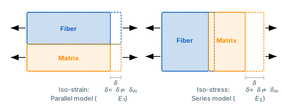
The simplest model. Under axial loading (parallel to fibers), fiber and matrix share the same strain. The composite stiffness is a volume-weighted average1:
This is exact for E1 and v12 under the assumption of perfect bonding. For E2 and G12, ROM uses the inverse (series) model, which treats fiber and matrix as springs in series:
The inverse model is a lower bound on the true transverse stiffness. It underestimates E2 because it ignores the constraint effects that arise from the cylindrical geometry of real fibers2. Use ROM as a quick check or a conservative estimate, not for final design values of E2 and G12.
Halpin-Tsai
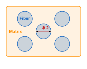
A semi-empirical improvement over ROM, widely used in industry1. It introduces a reinforcing efficiency parameter that accounts for fiber geometry:
Here P stands for the property being predicted (E2 or G12), and the reinforcing factor is set to for E2 (circular fibers) and for G12. E1 and v12 use the same ROM equations as above (Halpin-Tsai does not improve on these).
The parameter controls how effectively the fibers reinforce the matrix for a given loading mode. At the extremes, recovers the ROM parallel model (upper bound) and recovers the inverse series model (lower bound). For circular fibers, where a/b is the fiber cross-section aspect ratio in the loading plane (a/b = 1 for circles, so ). The lower value for G12 reflects that fibers constrain the matrix less under shear than under direct transverse tension.
Halpin-Tsai gives significantly better agreement with experimental data than inverse ROM, especially for glass/epoxy systems. It is a good default choice when you do not have test data to compare against.
Chamis (NASA TM-83696)
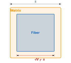
Developed by Christos Chamis at NASA Glenn Research Center3. The model assumes a square-root fiber packing arrangement rather than the series/parallel slabs of ROM:
The same square-root pattern applies to G12 (substituting shear moduli). E1 and v12 are again computed via ROM. Chamis tends to give slightly higher E2 predictions than Halpin-Tsai for typical carbon/epoxy systems, and is widely referenced in aerospace design guides.
Hopkins-Chamis elastic set (NASA TM-87154)
The parent model that Chamis simplifies. It takes the same square unit cell and splits it across the cell width into two regions acting in parallel: a bare-matrix strip of width that carries load on its own, and a fiber-bearing strip of width in which fiber and matrix act in series.
Drop the bare-matrix strip and what remains is the Chamis equation exactly. The strip's width falls steadily as Vf rises (at Vf = 0.10 roughly two thirds of the cell is bare matrix, and none of it is left as Vf approaches 1), but the gap between the two models does not follow that width, because the fiber-bearing strip it competes with stiffens at the same time. Hopkins-Chamis comes out below Chamis by in relative terms, which peaks at exactly Vf = 0.25 and tails off on both sides. For T300/5208 that is 15.5% on E2 at Vf = 0.10, 17.9% at 0.25, 15.8% at 0.45, 12.5% at 0.60 and 3.5% at 0.90, with the G12 gap a few points wider throughout. So the two models converge only on well-packed laminates, and differ across the whole mid-range where Chamis is known to run stiff. G12 follows the same pattern with shear moduli substituted, and E1 and v12 are again ROM.
The published equations look longer than this because TM-87154 was written for metal matrix composites at high temperature, where the fiber degrades from the outside in and grows an interphase. They therefore carry a third constituent and the ratio of current to virgin fiber diameter. An intact polymer composite is the zero-interphase case, in which those extra terms collapse and the two-constituent form above is what is left.
Puck semi-empirical model
Where the models above derive their form from an idealized geometry, Puck's model goes the other way: it starts from measured glass/epoxy moduli and fits analytical series forms to them9. This is the same Alfred Puck whose name is on the Puck failure criterion, but earlier work: these equations predict stiffness, not failure. The transverse modulus is:
The factor Em/(1 − vm²) is the plane-strain-stiffened matrix modulus: the fibers stop the matrix from contracting freely, so it responds stiffer than in a plain tension test. The 0.85 and the 1.25 exponent are the fitted part, with no geometric derivation behind them. In-plane shear uses the Förster/Knappe fit that Schürmann pairs with it (the package ships under Puck's name; strictly only the E2 equation is Puck's own):
E1 and v12 are again ROM. Being a fit, the model comes with a validity range: the curves were calibrated on glass/epoxy test data up to roughly Vf = 0.65. Inside that window and for that material system it is among the most accurate of the simple models, because it was fitted to exactly that data. Outside it the equations extrapolate, and for carbon fibers (whose transverse modulus is far lower than glass's) the extrapolation misbehaves in a way a derived model cannot: for T300/5208 the fitted E2 climbs past the fiber's own Ef2 before Vf = 0.70. Use it for glass/epoxy at realistic volume fractions; treat carbon predictions above Vf ≈ 0.5 with suspicion.
CCA (Composite Cylinders Assemblage)
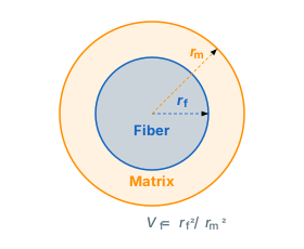
An exact analytical solution by Hashin and Rosen4, based on a model of concentric cylinders: a fiber core surrounded by a matrix annulus. Each cylinder pair is one fiber and its share of the surrounding matrix.
CCA gives the most rigorous prediction of G12 among the six models. For E1, v12, and the plane strain bulk modulus K23, CCA gives exact closed-form solutions8. The transverse modulus E2 then follows from the transverse isotropy relation:
The transverse shear modulus G23 is the one property CCA cannot pin down exactly, since the concentric cylinder geometry yields bounds rather than a single value. We use the Hashin lower bound, which is the tighter of the two for stiff-fiber/soft-matrix systems such as carbon/epoxy. E2 from CCA therefore tends to sit slightly below the Chamis prediction.
CCA is the recommended model when you need the highest accuracy for G12, or when comparing against other analytical bounds. In practice, all six models give similar E1 and v12 values. The differences show up primarily in E2 and G12.
Which elastic model should I use?
If you have experimental lamina data, compare each model's predictions against your test values and use the one that matches best for your material system. If you do not have test data:
- Halpin-Tsai is a safe default for most material systems.
- Chamis is widely used in aerospace and matches NASA design guide conventions.
- Hopkins-Chamis is the one to compare Chamis against, and worth running at any Vf a laminate is actually made at: for carbon/epoxy the bare-matrix strip it keeps is worth 12-18% on E2 across Vf = 0.10-0.60, and only falls to a few percent above roughly Vf = 0.85. The gap scales with 1 - Em/Ef2, so it is wider for glass/epoxy.
- Puck is the fitted one: for glass/epoxy up to about Vf = 0.65 it tracks test data closely, because it was calibrated on exactly that. For carbon, or beyond that Vf, it extrapolates and should not be trusted on its own.
- CCA gives the most rigorous G12 when that property matters (e.g. angle-ply laminates under shear).
- ROM is useful as a lower-bound sanity check, but should not be the sole basis for design.
ABD Composites lets you run all six models side by side in the UD lamina builder, so you can see exactly where they agree and where they diverge for your specific fiber/matrix combination.
Sweeping the fiber volume fraction
Every model above takes Vf as an input, and Vf is the single strongest lever on ply properties. Rather than guess a value and get one number per model, sweep Vf across its plausible range and watch all six models at once. Three things show up in the curves:
- E1 is a straight line, and all six models agree on it. The rule of mixtures is linear in Vf, and the other five inherit the same iso-strain argument for the fiber direction. If you only care about E1, the choice of model barely matters.
- E2 and G12 fan out. These are the matrix-dominated properties, where the models make genuinely different assumptions about how stress flows around the fibers. The spread in MPa grows with Vf because E2 itself does, so the curves visibly separate toward the right of the chart. As a percentage it is a different shape: the models are furthest apart across the low and middle range and only close up as Vf approaches 1. Either way the choice of model matters everywhere real laminates are made.
- v12 stays close to a straight line too, for the same reason as E1: Poisson contraction under axial load is strain-controlled, so a simple volume average captures it well.
Read the sweep at the Vf you can actually manufacture, not at the one that gives the nicest number. Hand layup typically lands around 0.40-0.50, wet filament winding and vacuum infusion around 0.50-0.60, and prepreg with autoclave cure around 0.55-0.65. Values above roughly 0.70 are not achievable with round fibers in practice, since the fibers would have to touch, leaving no resin to transfer load between them.

E₂ across the range, all six models. They stay within a few percent of each other up to about Vf = 40% and separate from there. Clicking in the plot sets the builder's Vf to the value you clicked.
The sweep is also the fastest way to sanity-check a supplier datasheet. Enter the fiber and matrix, find the datasheet's E2 on the chart, and see which Vf it implies. If that number is nowhere near the Vf the datasheet claims, either the constituent properties or the lamina properties are not what they say they are.
The fiber volume fraction page carries the same sweep for all twelve properties, grouped four to a section, along with what each manufacturing process achieves.
Strength Property Models
Predicting composite strength from constituents is much harder than predicting stiffness2. Stiffness is an elastic property that depends on the material's linear response. Strength involves failure: crack initiation, stress concentrations at the fiber-matrix interface, and mode-dependent failure mechanisms. No single model captures all of that accurately, so ABD Composites has four models, each predicting a different subset of the five lamina strengths.
The five lamina strengths
- S1t (F1t): longitudinal tensile strength. Fiber-dominated.
- S1c (F1c): longitudinal compressive strength. Fiber buckling/kinking.
- S2t (F2t): transverse tensile strength. Matrix-dominated.
- S2c (F2c): transverse compressive strength. Matrix-dominated.
- S12 (F6): in-plane shear strength. Matrix/interface dominated.
ROM Strength
Predicts longitudinal strengths (S1t, S1c) using volume-weighted averaging of fiber and matrix strengths. This works reasonably well for axial properties where fiber strength dominates. Requires fiber strengths (Sf1t, Sf1c) and matrix strengths (Smt, Smc). Note that the volume-weighted sum assumes fiber and matrix reach their ultimate strengths simultaneously, which over-predicts S1t. Treat it as an upper estimate.
Chamis Strength
Extends the square-root packing assumption to strength prediction3. Predicts transverse and shear strengths (S2t, S2c, S12) from matrix strength properties. Few models give you all three matrix-dominated strengths from one closed-form expression.
Tsai-Hahn
An empirical stress partitioning model5 that accounts for stress concentration at the fiber-matrix interface. Predicts transverse tensile strength (S2t) only. Useful when transverse tension is the critical failure mode and you want a second opinion beyond Chamis.
Hopkins-Chamis microbuckling strength
A compression-specific model6 that predicts longitudinal compressive strength (S1c) based on fiber microbuckling in the matrix. Uses the elastic properties (Gm, Gf12) rather than constituent strengths, so it needs no measured strength data at all.
Combining strength models
No single model predicts all five strengths. In practice, you combine results: ROM for S1t, Hopkins-Chamis for S1c, Chamis for S2t/S2c/S12. The UD lamina builder shows all model predictions side by side so you can pick the best value for each property. When measured lamina strength data is available, it should always take precedence over micromechanics predictions.

S₂ₜ across Vf, the two models that predict it. Transverse tensile strength falls as fiber content rises, because the matrix carries that load and there is less of it under sharper stress concentrations. Chamis and Tsai-Hahn agree at low Vf and part company above roughly 20%. See all four strength sweeps.
Thermal and Moisture Expansion
Composites expand and contract in response to temperature and moisture changes. Because fibers and matrix have very different expansion coefficients, the composite CTE and CME are strongly anisotropic: small in the fiber direction, much larger in the transverse direction.
Accurate CTE prediction matters for applications with thermal cycling (aerospace, satellite structures), cure stress analysis, and dimensional stability. CME matters when the laminate is exposed to humid environments (marine, outdoor structures).
CTE models
ABD Composites provides four CTE prediction models. All require the constituent CTEs (fiber: αf1, αf2; matrix: αm) plus the elastic constants used in the chosen elastic model.
- Schapery: The default model. Uses a stiffness-weighted ROM for the longitudinal CTE and a Poisson-corrected formula for the transverse CTE7:
- ROM: Simple volume-weighted average. Quick but less accurate for α2.
- Chamis: Uses the square-root packing assumption for improved transverse CTE prediction.
- CCA: Hashin-Rosen corrected CTE, accounting for the Poisson mismatch between fiber and matrix. Most rigorous, especially for carbon fibers where αf1 can be negative.

α2 across Vf, all four CTE models. The transverse direction is where they split: Chamis lowest, ROM in the middle, Schapery highest. CCA is drawn underneath Schapery, which is why three curves are visible rather than four. The axial CTE is the more striking plot: it passes through zero, so the ply stops expanding with temperature altogether.
CME (Coefficient of Moisture Expansion)
CME prediction uses the same equations as CTE, with moisture expansion coefficients (β) substituted for thermal expansion coefficients (α). For most fiber types (carbon, glass, boron), moisture absorption is negligible, so βf is effectively zero. The main exception is aramid fibers, which do absorb moisture.
What Inputs Do You Need?
The minimum inputs for elastic property prediction are:
- Fiber: Ef1, Ef2, Gf12, vf12
- Matrix: Em, Gm, vm
- Vf: Fiber volume fraction (typically 0.3 to 0.7)
Strength prediction additionally requires constituent strength values (which properties depend on the model). CTE/CME prediction requires the respective expansion coefficients. The UD lamina builder shows exactly which inputs are missing for each model and only displays results when the required data is available.
Fiber and matrix properties can be found in manufacturer datasheets, material databases, or textbook appendices. ABD Composites stores your fiber and matrix libraries so you can reuse them across projects.
The UD lamina builder: constituents and Vf on the left, the predicted lamina properties per model on the right.
From Micromechanics to Laminate Analysis
Micromechanics is the first step in the composite analysis workflow:
- Micromechanics: Fiber + matrix + Vf → lamina properties (E1, E2, G12, v12, strengths, CTE).
- Lamina builder: Save the predicted properties as a lamina in your material library.
- Laminate builder: Stack laminae at different angles and thicknesses to build a laminate.
- CLT: Compute the ABD matrix, engineering constants, ply stresses.
- Failure analysis: Check ply-level failure indices under load.
- Structural analysis: Evaluate beams, plates, panels, and cylinders.
For woven fabric composites, the micromechanics step feeds into a fabric homogenization step before entering the CLT pipeline. The fabric builder uses the same micromechanics models internally, but applies them at the yarn level and then integrates over the weave unit cell to get equivalent ply properties.
Which Micromechanics Model Should You Use?
All six models in ABD Composites take the same inputs: fiber properties, matrix properties, and fiber volume fraction. The difference is how they handle transverse and shear stiffness.
| Model | Strengths | Weaknesses |
|---|---|---|
| Rule of Mixtures (ROM) | Simplest; accurate for E1 and v12 | Significantly underestimates E2 and G12 (series lower bound) |
| Halpin-Tsai | Good for E2 and G12; widely used in industry | Reinforcement factor xi is empirical; must be calibrated |
| Chamis | Predicts all five elastic constants; good default choice | Slightly less accurate than CCA for high-stiffness fibers |
| Hopkins-Chamis | Chamis plus the bare-matrix strip, so softer in E2 and G12 at every Vf | Gap to Chamis peaks at Vf = 0.25 and closes only above Vf = 0.85; still 12-13% on E2 at Vf = 0.6 for carbon/epoxy, more for glass |
| Puck | Fitted to glass/epoxy test data, so the most accurate of the simple models inside that calibration range (Vf up to about 0.65) | Pure extrapolation outside it; for carbon/epoxy the fitted E2 overshoots badly at high Vf |
| CCA (Composite Cylinders Assemblage) | Most rigorous; provides upper and lower bounds | Same data requirements as others; marginal accuracy gain for most materials |
Author: Rick Schrijver
References
- Jones, R. M. (1999). Mechanics of Composite Materials, 2nd ed. Taylor & Francis.
- Roylance, D. (2000). Introduction to Composite Materials. MIT OpenCourseWare.
- Chamis, C. C. (1983). Simplified composite micromechanics equations for hygral, thermal, and mechanical properties. NASA TM-83696.
- Hashin, Z. & Rosen, B. W. (1964). The elastic moduli of fiber-reinforced materials. J. Applied Mechanics, 31(2), 223-232. doi:10.1115/1.3629590
- Tsai, S. W. & Hahn, H. T. (1980). Introduction to Composite Materials. Technomic.
- Hopkins, D. A. & Chamis, C. C. (1985). A unique set of micromechanics equations for high-temperature metal matrix composites. NASA TM-87154.
- Schapery, R. A. (1968). Thermal expansion coefficients of composite materials based on energy principles. J. Composite Materials, 2(3), 380-404. doi:10.1177/002199836800200308
- Barbero, E. J. (2011). Introduction to Composite Materials Design, 2nd ed. CRC Press, Section 2.3.4. doi:10.1201/9781439894132
- Schürmann, H. (2007). Konstruieren mit Faser-Kunststoff-Verbunden, 2nd ed. Springer, Chapter 8. doi:10.1007/978-3-540-72190-1
Frequently Asked Questions
Try it yourself
Build laminae from fiber and matrix properties, compare micromechanics models side by side, and save the results to your material library. It runs in the browser, with a free account and no install.
Create free account