
Bolted Joints in Composite Laminates
The loaded hole, the classical bearing, net-section and shear-out margins, and how the load splits between the fasteners in a row.
Bolted joints in composite laminates move load from one plate to the next through fastener holes. Every hole sees two loads at once: the bearing force its fastener pushes into the hole wall, and the bypass load the plate carries on past it toward the next fastener1. The Bolted Joint tool works out both for every fastener in the pattern from the plates, the bolt and the load you give it. Then it checks each hole twice: with the ply-by-ply point stress check the Open Hole tool uses, and with the classical hand margins for bearing, net-section tension, shear-out and fastener shear2.
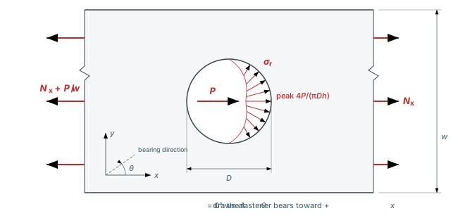
One loaded hole in a strip of width w, drawn at bearing angle θ = 0°. The fastener force P reaches the laminate as a cosine pressure σr over the half hole facing the bearing direction, peaking at 4P/(πDh). The plate carries the bypass Nx on past the hole and Nx + P/w behind it. The finite-width term P/(2w) takes the bypass to the average of the two3.
Everything on this page is in SI-mm: stresses in MPa, lengths in mm, running loads in N/mm, forces in N, angles in degrees counterclockwise from +x. The tool shows whichever units you have selected.
When to use this tool
Use the Bolted Joint tool when you have a joint rather than a single hole: two or three plates, a fastener pattern and one applied load. It shares that load between the rows and between the fasteners in each row, gives every composite plate's hole its own bearing force and bypass load, and checks all of them. You never type a bearing force in.
The Open Hole tool is the single-hole version, with the loads entered directly. Open-Hole Strength covers the stress field around an unloaded hole and the point stress criterion both tools use. The two tools share the Notch criterion settings (characteristic distance d0, finite-width correction, failure criterion and sweep resolution), so a d0 you calibrate in one carries straight over to the other. The tool covers mechanically fastened joints only. Bonded joints are outside its scope.
Inputs
A laminate card like every analysis tool, then a sketch of the joint and four groups of fields. The sketch is a plan of the overlap with every bolt drawn to scale, and a section through one bolt under it. Both redraw as you type. Each plate has its own colour, and the plates table below uses the same colours. The section shares one vertical scale between the plate stack and the bolt, so a bolt too short for its stack looks too short. After a run, a ring marks the governing bolt. A short line in each composite plate's colour, labelled 0°, shows the direction of its 0° plies. The sketch header holds the Rows and Columns steppers.
Load runs along x, and a row is a line of fasteners along x. Rows and Columns run from 1 to 5 each. The plan labels every dimension of the pattern: X, Sx, Z and Sz, plus the width W and the overlap, which follow from the pattern formulas below.
A single-lap joint with two rows of three bolts. The plan labels X, Sx, Z and Sz, and after a run a dashed ring marks the governing bolt.
Chips under the sketch show e/D against 2, S/D against 3, t/D against 1/3, the share of ±45° plies against 40%, and whether the threads clear the stack. The design-rule chips use the same thresholds and inputs as the result warnings, so they flag exactly the joints the warnings flag. The groups below the sketch:
- Bolt pattern: End edge distance X runs from the centre of the end bolt column to the plate end, and Column pitch Sx is the spacing between columns (with more than one column). Both run along the load. Side edge distance Z runs from the centre of the outer bolt row to the plate side edge, and Row pitch Sz is the spacing between rows (with more than one row). Both run across the load. Row offset (optional, with more than one row) shifts every even row along x. An edge distance no larger than D/2, or a row strip no wider than the hole, stops the analysis, and the field to change turns red. Edge distance factor, 1 by default, multiplies the bearing allowable of every composite plate (see Bearing knockdowns). It takes a value above 0 and at most 1. Below e/D 3, its info tooltip quotes test data for the tested layup closest to your plates.
- Plates: a Single lap, 2 plates or Double lap, 3 plates toggle, then a table with one row per plate, top to bottom. In a double lap, Plate 2 is the middle plate, and Plate 3 always matches Plate 1, so its row is locked. Each plate is Composite or Metal. A composite plate picks its layup from one list, with Laminate card (above) first and your saved laminates after it. Its thickness comes from that laminate and is read-only. It also takes a Bearing allowable (optional), the laminate bearing strength in MPa from an ASTM D5961 test4. Under its laminate sits the 0° direction field: the angle in degrees CCW from the load direction to the laminate's 0° plies, 0 by default. Set it for a plate whose 0° plies do not run along the load. The results then give that plate's ply angles from the load direction. A metal plate takes a Metal preset and a Thickness, and its allowable column reads N/A: a metal plate counts toward load sharing but gets no margins. An info icon in the metal select shows the preset's properties, with its CTE α.
- Fastener: Bolt metal is a preset. The info icon inside the select shows its E, ν, Ftu, Fsu and Fbru and the handbook source. Then come Diameter d, Shank length, Thread length, a Protruding or Countersunk Head, and Countersink depth, which you can edit once the head is Countersunk. A Countersunk head also adds Countersink factor, 1 by default, which multiplies the bearing allowable of Plate 1 and takes the same range, and a chip that warns when the countersink is deeper than 70% of Plate 1. The Fastener sleeve checkbox enables Sleeve metal and Outer diameter (= hole D). Without a sleeve, the hole diameter D equals the bolt diameter d.
- Load: Along the joint is the default. Joint load F per unit width in N/mm, negative for compression. The tool shares it equally between rows, and the spring network then splits each row's share between its fasteners. The line beside it gives the total F·W and the number of bolts. Temperature change ΔT is the service temperature minus the assembly temperature, 0 to leave it out. Its info tooltip lists each plate's CTE along x. With one bolt column, or plates with the same CTE along x, a warning says ΔT loads no bolt (see Compression and temperature change). Select At a point instead to load one plate with forces Px and Py in N and a moment M in N·mm (CCW positive), applied at a load point x, y in mm from the overlap corner. The loaded plate is Plate 1 in a single lap and Plate 2 in a double lap, and the other plates stay fixed. Load point x is 0 or more, and y runs from 0 to the overlap width W. The first time you select At a point, the load point starts halfway along the loaded plate's run-off as the sketch draws it, and halfway across the overlap. A line under the fields gives the bolt group centroid C and the moment about it. In this mode Edit positions turns the grid into a table of bolt positions, so you can move, add or remove bolts (up to 20). The table gives each bolt's nearest edge and e/D. Reset to grid, or a switch back to Along the joint, puts the bolts back on the grid. ΔT needs a load along the joint, so it is locked in this mode (see Load at a point).
- Notch criterion: Characteristic distance d0 starts at 1.5 mm. Its info tooltip explains why the check reads d0 out from the hole edge and how to calibrate it. The Finite-width correction switch is on by default. Characteristic distances rot and roc set the characteristic curve check. They have no default, and with either one blank that check reads N/A.
The failure criterion picker and the sweep resolution sit at the top of the results. The sweep sets how many stations go around each ring: 10°, 5° or 1°, which is 36, 72 or 360 stations. The tool runs one sweep per composite plate per bolt, so it starts when you stop typing and runs in the background. Until the new result is ready, the last one stays on screen under a progress bar. A 3-plate 5 × 5 pattern takes a few seconds at 5° and about five times as long at 1°.
There is no field for a fastener or sleeve shear allowable. Both come from the chosen preset's shear ultimate Fsu, and the bolt modulus Ef the load sharing uses comes from the same preset. The presets are Ti-6Al-4V, A-286, 17-4PH (H1025), 7075-T6 and 2024-T3, with values from MIL-HDBK-5J5.
Results
- Summary: Safety factor, the lowest across every bolt, plate and check, with SF = MS + 1 for the margin checks; Governing location, the plate and bolt (row, column) where it occurs, or a bolt column when fastener or sleeve shear governs; Governing check, one of Point stress criterion, Characteristic curve, Bearing, Net-section tension, Shear-out, Fastener shear or Sleeve shear. With a load at a point the bolts are numbered 1 to n instead of (row, column). An error alert shows when SF < 1.
- Plate and bolt: a picker above the tabs that lists every composite plate at every bolt. The Margins, Checks, Polar and Field tabs all show the one it names. It starts on the governing plate and bolt. When fastener or sleeve shear governs, it starts on the one with the lowest point stress SF.
- Margins tab: the point stress result for that plate and bolt: Point stress safety factor, Governing ply, Governing station and Governing mode (Failure mode when SF < 1). Station detail under it lists every ply at one station, ply 1 at the top, as on Ply Stresses & Strains. It opens on the governing station, and you can pick any other.
- Checks tab: Classical checks gives Bearing, Net-section tension and Shear-out for that plate and bolt, each with the applied stress, the allowable and MS. The info icon on each check gives its formula and where its allowable comes from. All plates and bolts follows, one row per plate per bolt, with columns Plate, Bolt (row, column), Bears toward, Point stress SF, Characteristic curve SF, Bearing MS, Net-tension MS and Shear-out MS, margins in percent. Bears toward is the bearing direction in degrees from x, and it is highlighted where a bolt bears away from the plate's loaded end. Hover over a bolt to see that plate's bearing force P and bypass Nx there, split into the parts from F and from ΔT under a temperature change. With a load at a point, a Load P column follows the bolt, the Point stress SF cell says whether the hole fails at the net section or the bearing face, and the rows sort by point stress SF within each plate. Click a row to show that plate and bolt in every tab. A last table gives Fastener shear and Sleeve shear.
- Polar and Field tabs: the margin sweep and the stress field of that plate's hole, the same views the Open Hole tool draws for its one hole. Click the field to pick a point. The tab then lists Nx, Ny and Nxy there, in that plate's laminate axes, and Use as analysis loads sends them to the laminate analysis pages.
The Checks tab for the 2 × 3 joint above. The Plate and bolt picker sets which case the classical checks show; the table under them covers every plate at every bolt.
A metal plate adds stiffness to the load sharing and gets no margins; its row in the table says so. The tables list the representative rows only: row 1, plus row 2 when a row offset is set. Why those two are enough is explained under plate sides below.
The Field tab for the governing plate and bolt. A click on the contour picks a point, and the readout at the cursor gives the value of the cell under it.
Key formulas
| Symbol | Name | Formula |
|---|---|---|
| σr | Cosine bearing pressure | |
| σ | Bearing and bypass superposition | |
| P/(2w) | de Jong finite-width term | |
| σbr | Bearing stress | |
| σnet | Net-section tension | |
| τso | Shear-out | |
| τb | Fastener shear | |
| τsl | Sleeve shear | |
| MS | Margin of safety | |
| W, overlap | Pattern dimensions | |
| C | Huth fastener compliance | |
| kseg | Plate segment stiffness |
- σr, cosine bearing pressure: The radial pressure (MPa) the fastener force P (N) puts on the hole wall, over the half hole facing the bearing direction. D is the hole diameter and h the laminate thickness, both in mm, and ϑ is measured around the hole from the bearing direction1,3.
- σ, superposition: The in-plane stress (MPa) at any point is the unloaded-hole field under the bypass running loads plus the loaded-hole field under P at bearing angle θ3.
- P/(2w), de Jong finite-width term: Half the bearing force smeared over the strip width w (mm), added to the bypass load in the bearing direction (N/mm)3.
- σbr, bearing stress: The bearing force over the projected hole area, in MPa2.
- σnet, net-section tension: The bypass Nbrg (N/mm) in the bearing direction across the strip, plus P, carried by the net section (w − D)h, in MPa2.
- τso, shear-out: The bearing force over two shear planes of length e (mm), the edge distance from the hole centre to the free edge, in MPa2.
- τb, fastener shear: The average shear stress (MPa) across the bolt, diameter d (mm), with ns shear planes: 1 for a single lap, 2 for a double lap2.
- τsl, sleeve shear: The average shear stress (MPa) across the sleeve's annulus, with outer radius ro = D/2 and inner radius ri the bolt radius, both in mm.
- MS, margin of safety: Each classical check's allowable over its applied stress, minus one. The tool shows it in percent2.
- W, overlap: The joint width and overlap length (mm) from the pattern: edge distances Z and X, row pitch Sz and pitch Sx.
- C, Huth fastener compliance: One fastener's shear flexibility in mm/N, from the plate thicknesses t1, t2 (mm), plate moduli Ex,1, Ex,2 and bolt modulus Ef (MPa), bolt diameter d (mm), shear planes n and Huth's joint constants a, b6.
- kseg, plate segment stiffness: The axial stiffness (N/mm) of one plate between two fasteners, from its modulus Ex (MPa) in the load direction, thickness t and strip width w (mm) and pitch Sx7.
The loaded hole: cosine bearing pressure
A fastener does not push on the whole hole wall. It bears on the half that faces the way it pushes, and the standard idealisation spreads its force P over that half as a radial pressure following a cosine1,3:
The angle ϑ runs around the hole from the bearing direction. The pressure peaks on the bearing axis at 4P/(πDh) and falls to zero at ±90°, as Figure 1 shows, and integrated over the half hole it gives back P. The cosine shape is an assumption. Real pin contact depends on the clearance between bolt and hole, on friction and on fit.
Solving it in the anisotropic plate
The loaded hole uses the same machinery as the unloaded one: the roots μ1, μ2 of the laminate's characteristic equation and the conformal mapping to ξk, both set out on Open-Hole Strength. What changes is the boundary condition. The cosine pressure is expanded in a Fourier series around the hole and truncated at 45 terms, the count Garbo and Ogonowski found sufficient1. A bearing load is not self-equilibrated on the hole boundary, because its reaction sits at infinity. So each stress function gains a logarithmic term, A ln ξ1 and B ln ξ2, whose constants come from a 4 × 4 real linear system8. The stress-function derivatives are then8:
Here Cm = (βm − μ2αm)/(μ1 − μ2) and Cm* = (βm − μ1αm)/(μ1 − μ2), built from the Fourier coefficients αm, βm of the pressure. The stresses follow from Φ1′ and Φ2′ with the same recovery formulas as the open hole.
Bearing direction
The solution is built for bearing along +x. For a bearing angle θ, measured counterclockwise from x, the compliance matrix [a] is rotated into the bearing frame, the problem is solved there, and the stresses are rotated back to x-y9. In the Bolted Joint tool you never enter θ. Plates on side A of the joint bear at 0° and plates on side B at 180°, as set out under load sharing below.
Bearing and bypass superposition
A hole in a joint carries both load paths at once. In a linear elastic plate their fields add3:
The first term is the unloaded-hole field under the bypass running loads, the second the loaded-hole field under P. In the Bolted Joint tool the bypass fed to each hole is Nx only: the load that plate still carries past that fastener, divided by the strip width w. The joint is loaded along x, so Ny and Nxy are zero.
Finite-width correction
The Lekhnitskii field assumes an infinite plate, where the fastener's reaction fades out at infinity. In a strip of width w it comes back as a mean membrane stress. With the Finite-width correction switch on, the tool adds half the bearing force, spread over the strip, to the bypass in the bearing direction3,1:
The sign follows the bypass component in the bearing direction, so a tension-reacted joint gains tension. Figure 1 shows where the term comes from: the plate carries Nx past the hole and Nx + P/w behind it, and Nx + P/(2w) is the average of the two. w here is the row's strip width (see strip width below). The same switch applies Tan's finite-width factor to an open hole, but every fastener in a joint carries a bearing load, so in the Bolted Joint tool the switch means the de Jong term only. The bypass past a loaded hole gets no factor for the narrow strip. The full note is under finite-width correction on Open-Hole Strength.
The point stress check at each hole
Each composite plate's hole then gets the point stress criterion, ply by ply: stations around the ring at r + d0, each ply's stress recovered there and tested with your failure criterion10,1. The lowest safety factor over every ply and station is that hole's point stress SF. The characteristic distance d0 is a calibration constant, and choosing d0 explains how to fit it to your own coupons.
The Polar tab at a 1° sweep: the point stress SF at each station around the governing hole.
Classical joint margins
Next to the field solution the tool runs the hand checks of joint design practice2. They take the same bearing force and bypass as the point stress check, and each gives a margin of safety MS = allowable/applied − 1, shown in percent.
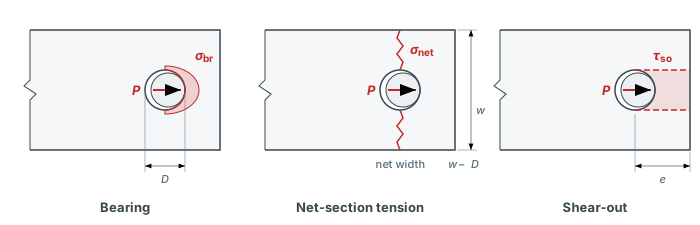
The three laminate failure modes, on an end hole with the fastener bearing toward the free edge. Bearing crushes the laminate in front of the fastener. Net-section tension breaks the ligaments either side of the hole, across w − D. Shear-out pushes a plug out along two planes of length e, measured from the hole centre.
Bearing
No CLT model predicts bearing strength. It is a laminate-level value from test, to ASTM D59614, and you enter it per plate as Bearing allowable (optional). Left blank, the bearing margin reads N/A. Bearing is the failure mode joint design aims for, because it is the ductile one: the edge distance and pitch rules below exist to push failure into bearing rather than shear-out or net-section tension2.
Bearing knockdowns
A bearing allowable from a standard test holds for a generous edge distance and a protruding head. A short edge distance or a countersunk head lowers it, and no model predicts by how much. So the tool takes two factors from you, both between 0 and 1: Edge distance factor ke for every composite plate, and Countersink factor kcs for Plate 1 when the head is countersunk. They act on the bearing margin only. Net tension, shear-out, fastener shear and the hole check do not use them.
A line above the margins table shows the product, for example "Bearing allowable 600.0 MPa × edge distance factor 0.740 × countersink factor 0.700 = 310.8 MPa used for Bearing MS." A factor at 1 is left out, and the copied table carries the allowable each case used.
The info tooltips on the two fields quote published tests, and they never set the factor. Below e/D 3, the edge distance tooltip reads a figure of bearing strength against e/D for three carbon/epoxy layups (30/60/10, 50/40/10 and 70/20/10 in % 0°/±45°/90°), each taken as a fraction of its value at e/D 516. At e/D 1.67 the 50/40/10 layup shows about 0.74 of that value. The tooltip picks the tested layup closest to each plate and names the plate where the value is lowest. Below e/D 1.5, the lowest tested point, it gives the e/D 1.5 value and says so. Countersunk heads give 25% to 35% lower bearing strength on quasi-isotropic carbon/epoxy17, and a countersink deeper than 70% of the plate is outside design guidance16. Use your own test data if you have it.
Net-section tension
Nbrg is the bypass component in the bearing direction, so the net section carries the bypass across the whole strip plus the bolt load, through the two ligaments either side of the hole2. The margin reads N/A when w ≤ D or when the net section is not in tension.
Shear-out
Two shear planes run from the hole to the free edge, and e is measured from the hole centre2. That is a deliberate choice, and the least conservative of the common forms. Others use the net length to the edge, 2(e − D/2)h. Taking e from the centre keeps shear-out on the same e as the e/D design rule. If you want the net-length form, enter e − D/2 as the edge distance.
Where the laminate allowables come from
Net-section tension and shear-out need laminate allowables, and the tool derives them instead of asking. The net-tension allowable is the laminate's unnotched first-ply-failure strength under uniaxial tension in the bearing direction. The shear-out allowable is the same under pure shear. Both use the failure criterion you picked for the point stress sweep, so they are membrane first-ply-failure estimates. A laminate keeps carrying load after its first ply fails (see Progressive Failure), which is why these allowables usually come out conservative against test-derived values.
Fastener and sleeve shear
ns is the number of shear planes the bolt carries the load across: 1 for a single lap (2 plates), 2 for a double lap (3 plates)2. d is the bolt's own diameter. The hole diameter D is the same unless a sleeve is fitted, and then D is the sleeve's outer diameter. The sleeve gets its own check on its annulus:
ro = D/2 is the sleeve's outer radius and ri the bolt radius, assuming the bolt fits the sleeve bore snugly. The ns factor is the tool's own assumption: the sleeve runs through the whole plate stack with the bolt, so each shear plane of a double lap cuts it too. Bolt and sleeve are each checked against the full bolt load P, with no split between them. Their allowables are the shear ultimate Fsu of the Bolt metal and Sleeve metal presets.
Two checks you can do by hand. A sleeve with P = 10 000 N, d = 6.35 mm and D = 7.94 mm has an annulus of π(3.972 − 3.1752) = 17.845 mm2, so τsl = 560.38 MPa in single shear and 280.19 MPa in double shear. The tool's default joint is one Ti-6Al-4V bolt with d = 6 mm in a single lap, load intensity 100 N/mm and X = Z = 15 mm. W = 2Z = 30 mm, so the bolt carries P = 3000 N and
against Fsu = 572 MPa for annealed Ti-6Al-4V bar5.
Strip width and pattern dimensions
Each row owns a strip of width w = Sz when there is more than one row, or w = W with a single row. That strip width feeds the net-section check, the P/(2w) term and the bypass Nx of every hole in the row. A strip width w ≤ D leaves no net section and blocks the analysis.
For an edge row, w = Sz overstates the width whenever Z < Sz/2, because that row has a neighbour on one side only and its true share toward the plate edge is Z. The tool does not flag this, so check the edge rows by hand when Z is small.
Load sharing between fasteners
Put several fasteners in a row and they do not share the load equally. Each fastener's own shear flexibility, and the stretch of the plates between fasteners, decide how much load transfers at each one6. The Bolted Joint tool shares the joint load equally between rows, then solves a spring network within each row.
Huth fastener flexibility
Huth's empirical formula gives the compliance of one fastener clamping two plates6:
t1 and t2 are the plate thicknesses, Ex,1 and Ex,2 their axial moduli in the load direction (1/(a11h) for a laminate, E for a metal plate, the same Ex as in kseg below), Ef the bolt modulus and n the number of shear planes. In Huth's words, "The bracket on the right side comprises the flexibility resulting from bearing loads, while the left part contains portions due to fastener bending and shear."6 C comes out in mm/N, and the fastener's shear stiffness is k = 1/C. The constants a and b depend on the joint group6:
| Joint group | a | b |
|---|---|---|
| I, bolted metallic joints | 2/3 | 3.0 |
| II, riveted metallic joints | 2/5 | 2.2 |
| III, bolted graphite/epoxy joints | 2/3 | 4.2 |
Every joint in the tool is bolted, so it uses group I for an all-metal joint and group III as soon as either plate is composite. The constants belong to the joint as a whole, not to one side of it.
Two details of the formula need care. The first is the third bracket term. The original print reads 1/(n t1Ef), but Huth's own calculated values only come out with 1/(2 t1Ef), which is how the formula is reprinted11. His single-shear specimen ISS01 has 2024-T3 plates with t1 = t2 = 5.1 mm and E = 72 000 MPa, and a Ti-6Al-4V bolt with d = 5.0 mm and Ef = 110 000 MPa (group I, n = 1). It gives C = 21.98 mm/MN with 1/(2 t1Ef) and 24.69 mm/MN with the printed term, and Huth's chart plots about 226.
The second is the plate order in double shear. In Huth's double-shear specimen, plate 1 is the middle plate carrying the full load and plate 2 is each outer plate carrying half. So for a double lap, t1 and Ex,1 belong to the middle plate, t2 and Ex,2 to one outer plate, and n = 2 scales the outer-plate terms for the pair. Specimen IDS01 (middle plate 5.1 mm, outer plates 2.5 mm, same materials) gives 9.12 mm/MN in that order, against about 9.2 on Huth's chart. The reverse order gives 11.476. In a single lap the order makes no difference.
With a sleeve fitted, the formula still takes the bolt's own d and Ef. Huth's specimens had no sleeves, so the sleeve only sets the hole diameter D. A real sleeved fastener is slightly stiffer than modelled, so the model spreads the load a little more evenly than the real joint does and slightly under-predicts the share the end fasteners carry.
The spring network
Within a row, each plate segment between two fasteners is an axial bar, and each fastener is a shear spring joining the two plates at its location:
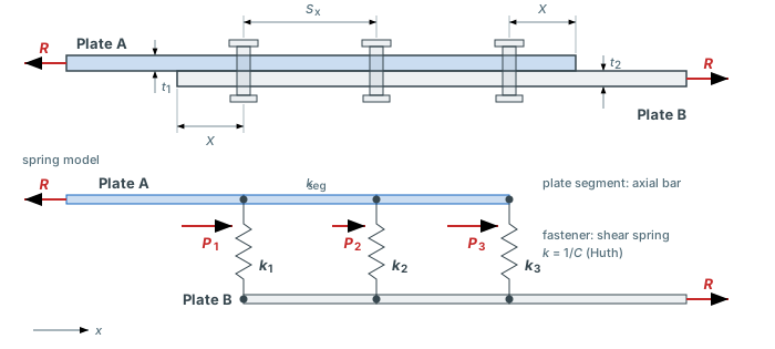
A single-lap row of three fasteners and the spring model behind it. Plate A is pulled toward −x and plate B toward +x, and the fasteners are numbered along +x. Plate segments are bars of stiffness kseg, fasteners are shear springs k = 1/C, and the end fasteners carry more than the middle one.
Ex is the plate's axial modulus in the load direction: Ex = 1/(a11h) from the laminate compliance [a] = [A]-1 of CLT7, or E for a metal plate. See Engineering Constants. A11/h would be wrong here. It is the laterally constrained modulus, which for a [±45]s laminate is more than twice Ex. In a double lap the two outer plates act as parallel bars between the same fasteners.
Plate A carries the row's full load into the joint and sheds it fastener by fastener; plate B starts unloaded and picks it up. The tool assembles this as a standard linear finite-element problem, bars plus springs, and solves it once. Each fastener's bearing force Pi and each plate's bypass past it come out of the same solve.
A two-fastener row shows how the split works. Take k = 105 N/mm for both fasteners, kA = 2 × 10⁵ N/mm for plate A's segment, kB = 105 N/mm for plate B's, and a row load R = 7000 N. Compatibility of the slips at the two fasteners gives
so P1 = 3000 N and P2 = 4000 N. The softer plate B stretches more between the fasteners, which relieves fastener 1 and pushes load onto fastener 2, at plate B's loaded end. With a single fastener there is nothing to share: it carries the whole row load and neither plate has any bypass. In a row of three with identical plates, the two end fasteners carry more than the middle one, and that is why end fasteners usually govern6.
The load sharing works in the load direction only. The laminate's biaxial and shear stiffness enter the point stress check that each P and bypass then feed, not the sharing itself. A double lap's outer plates must be identical, and the tool blocks one whose outer plates differ.
Plate sides, bearing angle and bypass
The network has two sides. Side A is Plate 1 of a single lap, or the middle plate (Plate 2) of a double lap. It is pulled toward −x, so the fastener bears on it toward its free end at +x: bearing angle 0°. Past fastener i it still carries the loads of the fasteners after it, the sum of Pj for j > i.
Side B is Plate 2 of a single lap, or the two outer plates (Plates 1 and 3) of a double lap. It is pulled toward +x and bears at 180°, and past fastener i it carries the sum of Pj for j < i. In a double lap the outer plates split side B's bearing force and bypass 50/50, while the middle plate takes the whole bolt load.
A row offset o shifts every even row by o along +x. Odd rows keep e = X on both sides. On an even row the side A plate's free edge moves o closer, e = X − o, and the side B plate's moves o further, e = X + o. Odd rows are all alike and even rows are all alike, so the tool analyses row 1, plus row 2 when a row offset is set. Those representative rows give the same governing result as analysing every row.
Compression and temperature change
A negative load intensity F is a compressive joint. The network is linear, so every bolt load and every bypass changes sign. A bolt then bears on side A at 180° and on side B at 0°. The bearing force keeps its size and the bypass becomes compressive.
A temperature change ΔT loads the bolts when the plates expand by different amounts, even with no applied load. Each plate's free strain is αxΔT, with αx the laminate's CTE along x from its membrane stiffness, or α for a metal plate. The tool solves the applied load and the temperature change as two separate spring networks and adds the bolt loads. The sign of each bolt's total load on a plate sets its bearing direction, so in one joint some bolts can bear toward the free end and others away from it. The results table shows the direction and the two parts of each bolt load. Every ply needs a CTE when ΔT is not 0. With one bolt column the plates expand freely about the bolts, and plates with the same CTE along x expand together, so in both cases ΔT loads no bolt and the tool says so under the field.
The safety factor scales the applied load only. The thermal part stays fixed, so a safety factor of 2 means twice F at the same ΔT. With F = 0 and ΔT not 0 there is nothing to scale, and the safety factor is the strength ratio on the thermal load. Net tension is N/A where the bypass is compressive or zero. Shear-out is N/A where the bolt bears away from the plate's free end, since there is no edge ahead of it to shear out to.
Load at a point
A bracket or a fitting rarely pulls straight along the joint. With At a point selected, the tool shares the load with the classical elastic centroid method instead of the spring network. It assumes rigid plates and bolts of equal stiffness. The origin is the overlap corner, x runs along the joint and y across it. The bolt group centroid C sits at the mean of the bolt positions, and the load moves to C as the same forces plus a moment:
Each of the n bolts takes Px/n and Py/n, plus a share of T in proportion to its distance from C, at right angles to the line from C:
Here rj is the distance from bolt j to C. Every bolt then bears in the direction of its own load: on the fixed plate along that load, on the loaded plate the opposite way. In a double lap, Plate 2 is the loaded plate, Plates 1 and 3 are fixed and split each bolt load 50/50. That split is this tool's reading of a double lap, since the classical method is written for one shear plane.
The 2 × 3 joint with the load at a point and Py = 500 N added. The sketch draws the load point, the centroid C and the moment line.
There is no bypass load in this mode, so each hole sees bearing only. Shear-out runs from the bolt along its bearing direction to the first overlap edge it reaches. It is N/A where that path leaves through the side where the plate carries on past the overlap, since there is no free edge there. Net tension uses the chord of the overlap through the bolt, across the bearing direction, shared by the holes that chord cuts. At 0° on a grid that is W divided by the rows, as in the along mode. These two rules at an angle are this tool's own reading of the classical checks, and no published case covers them. The results table says where each hole fails: at the net section when the governing station is more than 45° from the bearing direction, else at the bearing face.
The method does not model plate flexibility, fastener flexibility, bolt clearance or prying. The load sharing matches an independent implementation of the elastic centroid method to 1 part in 107.
Design-rule warnings
Some joint problems are not stress checks, so the tool warns about them rather than giving them a margin:
- Threads in bearing: the Shank length is shorter than the plate stack, so threads sit in the bearing surface, which the analysis does not model.
- Fastener bending: t/D above 1/3, where t is the thinnest plate (every plate of a double lap counts) and D is the bolt diameter. A thick plate on a thin bolt bends the bolt, which the margins do not include15.
- ±45° content: a composite plate with less than 40% of its thickness in plies at exactly +45° or -45° from the load axis. The angle includes the plate's 0° direction, and a fabric ply laid at ±45° counts fully. Metal plates are skipped15.
- e/D below 3, on the smallest modelled edge distance.
- S/D below 4, on the tighter of the spacings in use: Sx with more than one column, Sz with more than one row.
- A tight ligament: an interior fastener's shear-out path ends at the next hole, Sx − D/2 away. When that is shorter than the largest e, the interior fasteners' shear-out margin is overstated.
The e/D and S/D limits are Niu's minimums for a composite joint that fails in bearing rather than in shear-out or net tension2. Kassapoglou gives a pitch of 4D to 5D and an edge distance of at least 2.5D + 1.3 mm, so each hole stays close to an infinite plate15. None of the warnings blocks the analysis or changes a margin. The bearing knockdowns are your inputs (see Bearing knockdowns).
How the joint result is put together
- Row load = load intensity × W / rows, and each row's strip width w.
- Huth compliance of the fastener, then the spring network for the row: the bearing force Pi at each fastener and each plate's bypass past it.
- For every composite plate at every fastener in the representative rows: bypass Nx = plate bypass / w, bearing force Pi at 0° or 180°, the superposed field, the point stress sweep, the characteristic curve check when rot and roc are set, and the bearing, net-section tension and shear-out margins.
- Fastener shear and, with a sleeve, sleeve shear for each bolt.
- The Safety factor: the lowest of every point stress SF, every characteristic curve SF and every MS + 1, across all plates, bolts and checks.
A metal plate takes part in step 2 only. It adds stiffness to the load sharing and gets no margins.
Validation against published tests
Camanho and Lambert tested six double-shear joints in IM7-8552 [90/0/±45]3s, three bolted (B, clamped at 2.2 N·m) and three pinned (P), sized to fail in bearing, bearing/shear and net tension14. Each is a single fastener with no bypass, so the tool runs it as one loaded hole with the bearing along +x and the finite-width correction on. Ply stiffness and strength are the measured unidirectional values from their Tables 1 and 2. The tool does not model clamping, so a bolted specimen and its pinned twin get the same point stress prediction. Three columns of predictions:
- Defaults: the point stress check out of the box, max stress with d0 = 1.5 mm.
- Open-hole d0: the point stress check with d0 = 4.52 mm, the value fitted to their open-hole test OHT5 on Open-Hole Strength. A dash means it reaches past the strip edge.
- Characteristic curve: the tool's characteristic-curve check with the paper's own point-stress distances rot and roc (Table 16).
| Specimen | Failure mode | D (mm) | w/D | e/D | Test (MPa) | Defaults (MPa) | Error | Open-hole d0 (MPa) | Error | Curve (MPa) | Error |
|---|---|---|---|---|---|---|---|---|---|---|---|
| DSBFB | Bearing | 7 | 6 | 3 | 695.2 | 535 | −23.0% | 1145 | +64.7% | 636 | −8.5% |
| DSSFB | Bearing/shear | 6 | 6 | 2 | 701.8 | 576 | −17.9% | 1339 | +90.8% | 649 | −7.5% |
| DSTFB | Tension | 6 | 2 | 4 | 526.5 | 603 | +14.5% | – | – | 691 | +31.2% |
| DSBFP | Bearing | 7 | 6 | 3 | 706.3 | 535 | −24.3% | 1145 | +62.1% | 603 | −14.6% |
| DSSFP | Bearing/shear | 6 | 6 | 2 | 699.4 | 576 | −17.6% | 1339 | +91.4% | 594 | −15.1% |
| DSTFP | Tension | 6 | 2 | 4 | 460.5 | 603 | +30.9% | – | – | 624 | +35.5% |
Bearing strength σb = P/(D t), with t the laminate thickness. Sources: Camanho and Lambert Table 17 (experimental column), geometry Table 15, distances Table 16.
At the defaults the point stress check comes out 18 to 24 percent below the test for the bearing and bearing/shear specimens, the safe side. For the net-tension specimens, in w/D = 2 strips, it comes out 15 to 31 percent above, the unsafe side. On all six specimens the governing point is the bearing face (the 0° station, fibre compression in a 0° ply), so the check never looks at the net section where the narrow strips broke. A finite-width factor does not fix that. Applying Tan's factor to the bypass of these loaded holes adds tension past the hole, which relieves the bearing face and raises the predicted strength by about 3 percent. In a narrow strip, check net tension against an open-hole tension allowable from tests. The characteristic curve lands 8 to 15 percent below the test on bearing and bearing/shear.
The open-hole column is the warning. A d0 fitted on open-hole tests of the same laminate puts the bearing specimens 62 to 92 percent above the test. Do not carry an open-hole d0 over to a loaded hole.
Limitations
These bound what a safety factor above 1 means:
- Membrane only. The hole field and the plate moduli are built from [A]-1 alone7. For an unsymmetric laminate ([B] ≠ 0) an in-plane load also bends the plate, and the result is an approximation.
- No through-thickness effects. Delamination at the hole edge under bolt clamp-up, fastener bending and 3D bearing contact are all real bolted-joint failure modes, and none is analysed.
- One hole at a time. The spring network shares the load between fasteners, but each hole's stress field is solved on its own as a plane-stress membrane solution, with no stress interaction between neighbouring holes.
- Infinite plate. Finite width enters only through the de Jong P/(2w) term3. The bypass past a loaded hole gets no factor for a narrow strip. That is not why the w/D = 2 net-tension tests in the validation section come out high: the check fails them at the bearing face, not the net section.
- Cosine bearing pressure. The bearing force is applied as a cosine pressure over half the hole1. Real pin contact depends on clearance, friction and fastener fit.
- Knockdowns are inputs. The tool does not predict the bearing strength lost to a small e/D or a countersunk hole. You enter both factors, and they act on the bearing margin only.
- Open hole under compression. The hole check applies a compressive bypass to an open hole. A filled hole passes part of that load through the bolt, which the tool does not model, so the compressive hole check is conservative.
- Bearing-dominated joints. The point stress check at the bearing station is not validated for every joint. See below and the validation above.
The last item needs numbers. We ran the point stress check with the notch defaults both tools share (max stress, d0 = 1.5 mm, finite-width correction on), bearing along +x and no bypass load, against five published single-bolt pinned-joint tests12: D = 9.53 mm, e = 13.4 mm, widths from 19.0 to 38.0 mm, in a [±453/90/±452/04/90/04/±452/90/±453] carbon laminate13. The predicted failure loads came out 40 to 58 percent above the measured ones, worst on the narrowest strip. In every case the governing point was a shear mode in a 45° ply at the 0° station, right under the bearing peak. On the IM7-8552 double-shear tests above the same check was on the safe side for bearing and 15 to 31 percent high for net tension in narrow strips.
Author: Rick Schrijver
References
- Garbo, S.P. & Ogonowski, J.M. (1981). Effect of Variances and Manufacturing Tolerances on the Design Strength and Life of Mechanically Fastened Composite Joints. AFWAL-TR-81-3041, Air Force Wright Aeronautical Laboratories. (Cosine bearing pressure, 45-term series, ply-by-ply point stress check, finite-width term)
- Niu, M.C.Y. (1992). Composite Airframe Structures. Conmilit Press, Hong Kong. Chapter 5, §5.2. (Bearing, net-section and shear-out checks, fastener shear, edge distance and pitch design rules)
- de Jong, T. (1977). Stresses around pin-loaded holes in elastically orthotropic or isotropic plates. Journal of Composite Materials, 11(3), 313-331. doi:10.1177/002199837701100306
- ASTM D5961/D5961M. Standard Test Method for Bearing Response of Polymer Matrix Composite Laminates. ASTM International.
- U.S. Department of Defense (2003). MIL-HDBK-5J: Metallic Materials and Elements for Aerospace Vehicle Structures. Table 5.4.1.0(c1). (Ti-6Al-4V shear ultimate Fsu = 572 MPa)
- Huth, H. (1986). Influence of fastener flexibility on the prediction of load transfer and fatigue life for multiple-row joints. In J.M. Potter (ed.), Fatigue in Mechanically Fastened Composite and Metallic Joints, ASTM STP 927, ASTM International, pp. 221-250. Eq. 1 p. 235; Tables 2-3 pp. 228-229; Figs. 8-9 pp. 237-238. doi:10.1520/STP29062S
- Jones, R.M. (1999). Mechanics of Composite Materials, 2nd ed. Taylor & Francis. Chapter 4. (Laminate compliance, Ex from [A]-1)
- Lekhnitskii, S.G. (1968). Anisotropic Plates, 2nd ed., transl. S.W. Tsai and T. Cheron. Gordon and Breach. Eq. 37.2-37.6. (Loaded-hole stress functions and the logarithmic term)
- Esp, B. (2007). Stress Distribution and Strength Prediction of Composite Laminates with Multiple Holes. PhD thesis, University of Texas at Arlington. Eq. 9.6. (Rotation of the compliance matrix into the bearing frame)
- Whitney, J.M. & Nuismer, R.J. (1974). Stress fracture criteria for laminated composites containing stress concentrations. Journal of Composite Materials, 8(3), 253-265. doi:10.1177/002199837400800303
- Gunbring, F. (2008). Prediction and Modelling of Fastener Flexibility Using FE. MSc thesis, Linköping University, LIU-IEI-TEK-A--08/00379--SE. DiVA diva2:17841. (Reprints Huth's formula and constants)
- Aluko, O. (2011). An analytical method for failure prediction of composite pinned joints. Proceedings of the World Congress on Engineering 2011, London, 6-8 July 2011, pp. 2581-2587. Lecture Notes in Engineering and Computer Science. Paper (PDF)
- Kweon, J.H., Ahn, H.S. & Choi, J.H. (2004). A new method to determine the characteristic lengths of composite joints without testing. Composite Structures, 66(1-4), 305-315. doi:10.1016/j.compstruct.2004.04.053
- Camanho, P.P. & Lambert, M. (2006). A design methodology for mechanically fastened joints in laminated composite materials. Composites Science and Technology, 66(15), 3004-3020. doi:10.1016/j.compscitech.2006.02.017 (Tables 1-2, IM7-8552 ply data; Tables 15-17, double-shear joint tests and characteristic distances)
- Kassapoglou, C. (2013). Design and Analysis of Composite Structures, 2nd ed. Wiley. Section 8.7 and Chapter 12, Figure 12.1. (Fastener bending, ±45° ply content, edge distance and pitch)
- Ramkumar, R.L., Saether, E.S. & Cheng, D. (1986). Design Guide for Bolted Joints in Composite Structures. AFWAL-TR-86-3035, Air Force Wright Aeronautical Laboratories. (Fig. 20, bearing strength against E/D; Section 2.5.1, countersink depth)
- Camanho, P.P. & Tong, L. (eds) (2011). Composite Joints and Connections. Woodhead Publishing. Chapter 3. (Countersunk-head bearing strength)
Frequently Asked Questions
Try it yourself
Check a joint of your own with the Bolted Joint tool: the load on every fastener, the classical margins for every plate and bolt, and the point stress check at the governing hole. It runs in the browser, with a free account and no install.
Create free account