
Open-Hole Strength of Composite Laminates
The stress concentration around a circular hole in an anisotropic laminate, and the point stress criterion that turns it into a notched strength check.
A hole cuts load-carrying fibres, and the load they carried has to flow around it. The open-hole strength of a composite laminate is the load at which that detour breaks something. Right at the hole edge the stress peaks at several times the far-field value1, but laminates do not fail at the elastic peak: a little damage near the edge relieves it. So the Open Hole tool reads the stress a short distance d0 outside the edge, checks every ply there against your failure criterion, and reports the load multiplier to first ply failure3.
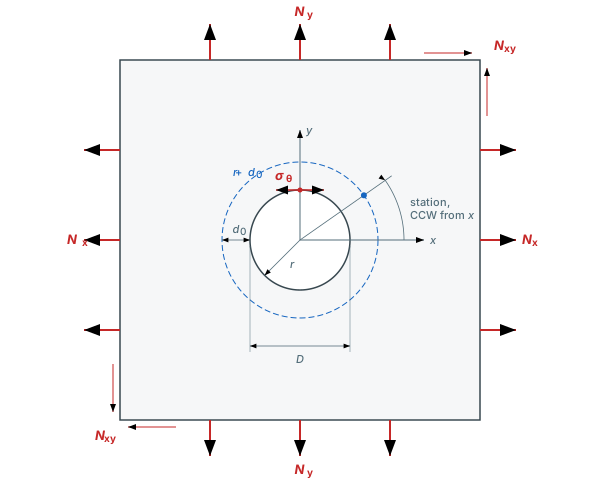
A hole of diameter D in a plate under remote running loads. The tool evaluates each ply on the dashed ring at radius r + d0, one station at a time, with station angles measured counterclockwise from x. Under Nx the peak hoop stress σθ sits at the hole edge 90° from the load.
Everything on this page is in SI-mm: stresses in MPa, lengths in mm, running loads in N/mm, forces in N, angles in degrees counterclockwise from +x. The tool shows whichever units you have selected.
When to use this tool
Use the Open Hole tool for a single hole with the loads typed in directly: cutouts, access holes, lightening holes, and fastener holes where you already know the bypass load flowing past and, if there is one, the bearing force the fastener puts in. It answers one question. At what multiple of these loads does the first ply fail near the hole?
The Bolted Joint tool runs the same single-hole check, but it works out the loads for you first. It splits the applied load across its plates and bolts, then checks every hole the way the Open Hole tool checks one. Bolted Joints covers how it shares the load and the classical margins it adds. The two share the Notch criterion settings (characteristic distance d0, finite-width correction, failure criterion and sweep resolution), so a d0 you calibrate in one carries straight over to the other. The ply check itself is any criterion from Failure Criteria.
Inputs
A laminate card like every analysis tool, then a sketch of the hole and four groups of fields. The sketch is a plan of the strip drawn to scale, with an edge view under it, and it redraws as you type. With w blank the strip edges draw dashed and the caption reads "No width: infinite plate". With e blank both ends draw as breaks; once you enter e, the free edge sits at the +x end for every bearing angle, and only the P arrow turns. With a bearing load at any θ other than 0°, a chip notes that the analysis measures e along θ and w across it. A dashed ring at r + d0, with r the hole radius, marks where the point stress criterion checks each ply. Click into a geometry or load field and its dimension or arrow turns blue on the sketch.
Chips under the sketch show w/D against 4, e/D against 3 and the load case (Unloaded hole, Bearing only, Bypass only, or Bearing + bypass). When w or e is blank, a chip says which check reads N/A instead. The groups below the sketch:
- Geometry: Hole shape, Circle or Ellipse (see Elliptical holes below). For a circle, Hole diameter D, then Width w (optional) and Edge distance e (optional). w is the strip width or fastener pitch. The net-section tension margin and the finite-width correction use it, and a blank w means an infinite plate. e runs from the hole centre to the free edge in the bearing direction, and the shear-out margin uses it.
- Loads: two rows. The Bypass row takes Nx, Ny and Nxy in N/mm: the running loads that flow past the hole, measured far from it, with tension positive. The Bearing row takes the Bearing force P in N, the load a fastener transfers into the laminate, and the Bearing angle θ, the direction the fastener pushes on the hole in degrees counterclockwise from x. P = 0 gives an unloaded open hole, and θ = 0° bears along +x. The 0°, 90°, 180° and 270° buttons set θ in one click.
- Allowables: Bearing allowable (optional) is the laminate bearing strength from an ASTM D5961 test11, and Fastener shear allowable (optional) is the shear ultimate of the fastener material. A blank allowable shows its check as N/A.
- Notch criterion: Characteristic distance d0 starts at 1.5 mm, and d0 = 0 evaluates the hole edge itself. Its info tooltip explains why the check reads d0 out from the hole edge, gives the literature band for carbon/epoxy and says how to calibrate it. The Finite-width correction switch is on by default. Characteristic distances rot and roc set the characteristic curve check for a loaded hole. They have no default, and with either one blank that check reads N/A.
The failure criterion picker sits on the Margins and Checks tabs, and the sweep resolution on the Margins tab. The sweep sets how many stations go around the ring: 10°, 5° or 1°, which is 36, 72 or 360 stations. The sweep starts when you stop typing and runs in the background. Until the new result is ready, the last one stays on screen under a progress bar.
A 6 mm hole in a 36 mm strip, with 100 N/mm bypass and a 1000 N bolt load along +x. The sketch draws the strip to scale, and Station detail on the Margins tab lists every ply at the station you pick.
Results
- Margins tab: Safety factor, the minimum load multiplier to first ply failure on the ring at r + d0 across all plies and stations; Governing ply, with ply 1 at the top; Governing station, the angle around the hole counterclockwise from x; Governing mode, which reads Failure mode with an error alert when SF < 1. Characteristic curve SF follows, with the governing ply, its station and whether that means net tension or shear-out or bearing, or a line saying why the check is N/A. It is a separate verdict: the Safety factor above is the point stress result alone. Station detail lists every ply at any station you pick.
- Checks tab: the classical margins, the hand checks for Bearing, Net-section tension, Shear-out and Fastener shear, each with its applied stress, allowable and MS. The info icon on each check gives its formula and where its allowable comes from.
- Polar tab: two views around the ring. Safety factor plots the lowest ply SF at each station. Tangential stress plots the laminate stress along the hole edge at each station, which for a circle is the hoop stress σθ on the r + d0 ring.
- Field tab: stress or strain maps around the hole, in global axes or in one ply's local axes, with the hole at the origin and the axes in hole diameters. A dashed curve marks where the point stress check reads, d0 out from the hole edge, and a ringed dot labelled with its angle marks the governing station. Click the field to pick a point. The tab then lists Nx, Ny and Nxy there, in the laminate axes, and Use as analysis loads sends them to the laminate analysis pages.
The Checks tab for the same hole. Each classical margin has its applied stress, its allowable and MS, and the governing check is marked.
The tool does not print a stress concentration factor Kt. Kt is theory you check the results against, and the Tangential stress view is where you check it: set d0 to 0 and the ring sits on the hole edge.
The Tangential stress view for the same hole, read on the ring at r + d0. Under Nx the peaks sit near 90° and 270°, at right angles to the load.
Key formulas
| Symbol | Name | Formula |
|---|---|---|
| μ1, μ2 | Characteristic equation | |
| σ∞ | Remote stress | |
| Kt (isotropic) | Kirsch stress concentration | |
| Kt (orthotropic) | Orthotropic stress concentration | |
| P/(2w) | de Jong finite-width term | |
| PSC | Point stress criterion |
- μ1, μ2, characteristic equation: A quartic in the laminate's thickness-normalised membrane compliance [a] = h[A]-1. Its two roots in the upper half-plane carry all of the laminate's anisotropy into the hole solution1.
- σ∞, remote stress: The solution works in stresses, so each bypass running load (N/mm) is divided by the laminate thickness h (mm) to give an average stress in MPa.
- Kt, isotropic: Peak hoop stress at the hole edge over the remote stress, for an isotropic plate in uniaxial tension2. The peak sits 90° from the load.
- Kt, orthotropic: The same ratio for an orthotropic laminate loaded along its x axis, from the laminate engineering constants1.
- P/(2w), de Jong finite-width term: Half the bearing force smeared over the strip width and added to the bypass load in the bearing direction (N/mm)5.
- PSC, point stress criterion: Failure is predicted when the stress at distance d0 (mm) outside the hole edge reaches the unnotched strength3.
The stress field around an unloaded hole
The tool solves the hole with Lekhnitskii's complex-variable method for anisotropic plates1, in the closed form Esp gives for laminates4. The laminate enters through one matrix. Take the membrane compliance [A]-1 from CLT, multiply by the thickness to get [a] = h[A]-1, and substitute its terms into the characteristic equation above. Its four roots come as two complex-conjugate pairs. The two with positive imaginary part, μ1 and μ2, define the complex coordinates zk = x + μky in which the whole field is written.
Conformal mapping
A circle is an awkward boundary in zk, so each point is mapped to a coordinate ξk in which the hole edge becomes the unit circle1,4:
The sign is picked per point so that |ξk| ≥ 1. Every point in the plate lands on or outside the unit circle. A point inside the hole has no valid mapping, and no stress.
Stress recovery
With Φk′ the derivatives of the two stress functions, the in-plane stresses are1:
For an unloaded hole the stress functions follow from the remote stresses σx∞ = Nx/h, σy∞ = Ny/h and τxy∞ = Nxy/h4:
These stress functions carry only the disturbance the hole causes. The total stress is the recovered field plus the remote stress, which is why the field settles back to N/h a few diameters away. When you enter a bearing force P, the tool superposes a second, loaded-hole field on top of this one, and the two add5.
The Field tab for the hole under bypass only: σx in global axes, with the axes in hole diameters. The stress concentrates above and below the hole and falls back toward Nx/h away from it.
Orthotropic stress concentration factor
For an orthotropic laminate (A16 = A26 = 0) loaded along x, the peak hoop stress sits at the hole edge 90° from the load, and its ratio to the remote stress has a closed form1:
Ex, Ey, Gxy and νxy are the laminate's membrane engineering constants. The formula rewards stiffness along the load and punishes a soft shear modulus. A stiff fibre direction pulls load toward the hole edge, where those fibres have been cut, instead of letting it spread sideways through the matrix.
Take a single 0° unidirectional carbon ply with E1 = 140 000 MPa, E2 = 10 000 MPa, G12 = 5 000 MPa and ν12 = 0.3, loaded along the fibres. Then Ex/Ey = 14 and Ex/Gxy = 28, and
More than twice the isotropic value. Practical layups fall roughly between 3 and 9, and an ideal quasi-isotropic laminate comes back to exactly 3. For a laminate that is not orthotropic, or under combined load, there is no closed form. The full field above still applies, and the Tangential stress view shows the result.
The isotropic limit: Kt = 3
For an isotropic plate under remote uniaxial tension, the hoop stress at the hole edge 90° from the load is three times the remote stress. This is the Kirsch solution2. In the anisotropic method it is a degenerate case: the characteristic equation collapses to (μ2 + 1)2 = 0, a repeated root μ = i, and the coefficients Ck divide by μ1 − μ2. The tool separates the two roots by a tiny amount and takes the isotropic answer as the limit of the anisotropic one, so the same code path serves both.
That makes it the check to run before you trust anything else. In the Open Hole tool:
- Make an isotropic lamina: E1 = E2 = 70 000 MPa, ν12 = 0.3, G12 = E/(2(1 + ν)), strength 1000 MPa in every direction.
- Lay up one 1 mm ply, so h = 1 mm.
- Set D = 6 mm, Nx = 100 N/mm, every other load zero, d0 = 0, and pick the max stress criterion.
The Tangential stress view should read 3Nx/h = 300 MPa at 90°, and the Safety factor should be 1000/300 = 3.333 at the 90° station. If your own laminate gives numbers you cannot explain, come back to this case first.
Finite-width correction
The Lekhnitskii solution assumes an infinite plate. In a strip of width w the bypass load has to squeeze through the net section beside the hole, so the stress there runs higher than the infinite-plate field says. With the Finite-width correction switch on and P = 0, the tool multiplies the bypass Nx by Tan's finite-width factor KT/KT∞ before it solves the field6. Because the field is linear in the load, that scales the whole Nx field by the same factor. Ny and Nxy are not scaled: the strip has no width limit along its length.
For a circular hole in an orthotropic laminate the factor is Tan's improved orthotropic form (his Eq. 24). Any other laminate, and every ellipse, uses his anisotropic form (Eq. 21), which needs the laminate's complex roots. Both reduce to Heywood's formula for an isotropic plate18:
KT/KT∞ = [2 + (1 − D/w)3] / [3(1 − D/w)]
That is 1.08 at w/D = 4 and 1.42 at w/D = 2. Tan's factor is exact at the hole edge and approximate away from it. Nguyen-Hoang and Becker compared it with an exact finite-plate solution at w/D = 317: within the first fifth of the net section, where the check point sits, it was 2% high for a quasi-isotropic laminate and 10% low for [±45]s. Far from the hole the scaled field overstates the remote stress by the factor itself, and the Field tab shows that at its edge.
A loaded hole (P > 0) gets the de Jong term instead. In an infinite plate the fastener load fades out at infinity, but in a strip of width w it comes back as a mean membrane stress, so the tool adds half the bearing force spread over the strip, ±P/(2w), to the bypass load in the bearing direction5. The sign follows the bypass component in that direction, so a tension-reacted joint gains tension and a compression-reacted joint gains compression. Tan's factor does not act on a loaded hole, with or without bypass: it was derived for a remote load past an unloaded opening. With the width left blank neither correction runs.
Notched strength: the Whitney-Nuismer point stress criterion
Divide the unnotched strength by Kt and you get a notched strength well below what open-hole tests measure. Real laminates relieve the elastic peak with subcritical damage before the hole edge fails. Whitney and Nuismer's point stress criterion accounts for this empirically: it predicts failure when the stress at a fixed characteristic distance d0 outside the hole edge reaches the unnotched strength3.
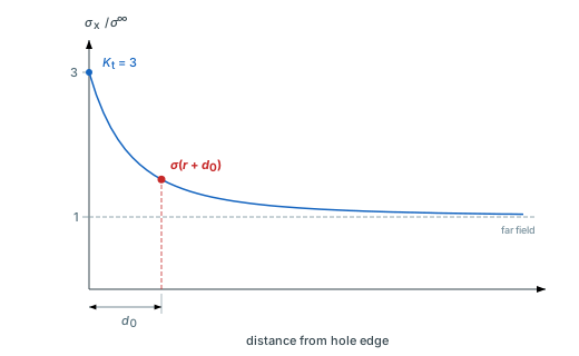
The isotropic Kirsch field ahead of the hole2. The stress starts at Kt = 3 on the edge and decays toward the far-field value. The point stress criterion reads it at d0, where it is already well below the peak.
The criterion also explains the hole-size effect. The stress gradient scales with the hole radius, so for a fixed d0 a small hole has shed most of its peak by the time you reach the ring, while a large hole has barely started. Two holes with the same Kt therefore have different notched strengths, and the larger hole is the weaker one3.
How the tool applies it, ply by ply
Whitney and Nuismer applied the criterion at laminate level, comparing a laminate stress with a laminate strength3. The Open Hole tool works one ply at a time instead, the way the mechanically fastened joint analysis of Garbo and Ogonowski does7:
- Place stations around the ring at r + d0, at the sweep resolution you picked.
- At each station, take the laminate stress from the field above and convert it to midplane strain with membrane CLT, ε = [A]-1N.
- Recover each ply's stress, σk = [Q̄]kε, and rotate it to the ply axes8, as on Ply Stresses & Strains.
- Apply the chosen failure criterion with the ply's unnotched strengths.
- Report the minimum safety factor over every station and ply, with the ply, station and mode where it occurs.
The answer is first ply failure on the ring, with your own criterion deciding what failure means, and it tells you which ply and which mode to fix. The tool does not compute the laminate-level closed-form notched strength. For how a laminate carries on after its first ply fails, see Progressive Failure.
Choosing d0
d0 is a calibration constant, not a material property. No theory predicts it. For carbon/epoxy quasi-isotropic laminates, literature values cluster between 0.5 and 2.0 mm; the tool starts at 1.5 mm, a common first guess, and Whitney and Nuismer's own value was 1.0 mm3. The result is sensitive to it. A larger d0 puts the ring further down the stress gradient and predicts a higher notched strength, so an unjustified large value is unconservative.
Calibrate it against your own open-hole tension coupons, tested to ASTM D576610: model the coupon in the tool, then adjust d0 until the predicted failure load matches the test. Only then size anything with it. The related average stress criterion, which averages the stress over a distance instead of reading it at a point, is not implemented.
The characteristic curve check
A loaded hole fails differently at its sides and under the fastener, and one ring at r + d0 treats both the same. Camanho and Lambert's characteristic curve uses two distances instead15: rot at 90° to the bearing direction, where the net section fails in tension, and roc along the bearing direction, where the fastener crushes the laminate. The tool runs it beside the point stress check, never instead of it, for a loaded circular hole only. The Open Hole and Bolted Joint tools both use it.
R is the hole radius and φ is measured from the bearing direction. Only the half facing the bearing load is swept, at the same sweep resolution as the point stress check. At each station the tool recovers every ply's stress from the same superposed field and checks it with a fibre criterion, the modified Yamada-Sun criterion15, whatever failure criterion you picked. In-plane shear lowers the compressive fibre strength but not the tensile one:
The lowest safety factor over every station and ply is the Characteristic curve SF. The angle of the governing station names the failure mode: 75° to 90° from the bearing direction is net tension, anywhere else is shear-out or bearing.
The check reads N/A in four cases:
- rot or roc is blank.
- The hole has no bearing load.
- The curve reaches past the strip edge or the free edge. The rot and roc fields then turn red, and the point stress check still runs.
- The hole is an ellipse.
Like d0, rot and roc are calibration constants, so the fields have no default. Camanho and Lambert's design charts fit one material and one layup, and the tool does not apply them. Three things differ from the paper. SL is the ply's unidirectional shear strength, not the in-situ value, which is conservative. Only the point form is implemented, not the average stress form. And the criterion checks fibres only, so a matrix-dominated weak spot can look stronger here than under the point stress check with an interactive criterion. The paper calibrated its distances on a finite element stress field, so distances taken from its tables give lower safety factors here than the paper reports. On published double-shear joint tests the check comes out 8 to 15 percent below the test for bearing and bearing/shear failures (see Bolted Joints validation).
Elliptical holes
Set Hole shape to Ellipse and the tool analyses an elliptical cutout instead of a round hole. Enter Hole length 2a, Hole height 2b and Hole angle ψ, the angle counterclockwise from the laminate x axis to the length. 2b can be larger than 2a: that is the same ellipse turned 90°. The ellipse is an open hole only. It carries no bearing load.
The method is the same Lekhnitskii solution as for the circle1, with semi-axes a along the length and b across it. Only the mapping and the loading constants change:
Set a = b = r and these become the circle's equations above. A turned hole is solved in its own axes: the tool turns the laminate compliance and the remote load by ψ, solves, and turns the stresses back. The isotropic case has a closed form. Under uniaxial tension across the hole length, the stress at each end of the length is Kt = 1 + 2a/b times the remote stress13: 3 for a circle, 5 for 2a/2b = 2, 9 for 2a/2b = 4. The sharper the ends, the higher the peak.
The point stress check reads each ply d0 out from the hole edge along the edge normal, so the checked points trace a curve parallel to the hole rather than a ring. Stations are still spaced by the angle around the hole centre, counterclockwise from x, and Governing station and the Polar tab read in that angle. Net-section tension uses H, the span of the hole across the strip, in place of D:
A chip under the sketch shows w/H and H. Keep w/H at 4 or more, for the same reason as w/D for a circle. The d0 curve has to stay inside the plate, so d0 must be less than w/2 − H/2, and less than e minus the distance the hole reaches along x.
With Ellipse selected, the bearing force and angle, both allowables and the characteristic distances rot and roc are switched off. Bearing, shear-out and fastener shear show N/A, and so does the characteristic curve check. The tool keeps the values you entered, so they come back when you switch to Circle. The finite-width switch stays on: Tan's factor covers ellipses, with 2a taken as the hole's span H across the strip. A turned ellipse gets the factor of the unturned ellipse with the same span and length along x, an approximation Tan's paper does not cover.
The hole-edge stresses are cross-checked against an independent implementation on ellipses from 2a/2b = 1/3 to 4, turned and not, including an unbalanced layup, and agree to better than one part in a million.
Validation against published tests
We ran the Open Hole tool on 15 published open-hole tension tests in IM7-8552 carbon/epoxy: Camanho and Lambert's nine specimens15, two smaller holes from Camanho et al.16, both in [90/0/±45]3s, and Green et al.'s four [45/90/−45/0]4s specimens, also from Camanho et al. Ply stiffness and strength are the measured unidirectional values from Camanho and Lambert's Tables 1 and 2, and the finite-width correction is on. Two columns of predictions:
- Defaults: what the tool gives out of the box, max stress with d0 = 1.5 mm.
- Fitted d0: d0 = 4.52 mm, fitted so the tool matches OHT5 exactly, then used unchanged on every other row. It is the calibration the d0 input asks you to do with your own coupons. A dash means the fitted d0 reaches past the strip edge, which the tool blocks.
| Specimen | Layup | D (mm) | w/D | Test (MPa) | Defaults (MPa) | Error | Fitted d0 (MPa) | Error |
|---|---|---|---|---|---|---|---|---|
| OHT1 | [90/0/±45]3s | 6 | 2 | 252.2 | 227 | −10.0% | – | – |
| OHT2 | [90/0/±45]3s | 6 | 4 | 372.8 | 298 | −20.1% | 385 | +3.3% |
| OHT3 | [90/0/±45]3s | 6 | 6 | 438.7 | 311 | −29.1% | 402 | −8.4% |
| OHT4 | [90/0/±45]3s | 8 | 2 | 247.3 | 204 | −17.5% | – | – |
| OHT5 | [90/0/±45]3s | 8 | 4 | 366.6 | 269 | −26.6% | 367 | +0.1% |
| OHT6 | [90/0/±45]3s | 8 | 6 | 375.7 | 281 | −25.2% | 383 | +1.9% |
| OHT7 | [90/0/±45]3s | 10 | 2 | 260.8 | 189 | −27.5% | 267 | +2.4% |
| OHT8 | [90/0/±45]3s | 10 | 4 | 344.5 | 249 | −27.7% | 351 | +1.9% |
| OHT9 | [90/0/±45]3s | 10 | 6 | 373.7 | 260 | −30.4% | 366 | −2.1% |
| C12-d2 | [90/0/±45]3s | 2 | 6 | 555.7 | 401 | −27.8% | 456 | −17.9% |
| C12-d4 | [90/0/±45]3s | 4 | 6 | 480.6 | 352 | −26.8% | 427 | −11.2% |
| G-3.175 | [45/90/−45/0]4s | 3.175 | 5 | 478 | 364 | −23.8% | 432 | −9.6% |
| G-6.35 | [45/90/−45/0]4s | 6.35 | 5 | 433 | 301 | −30.5% | 392 | −9.5% |
| G-12.7 | [45/90/−45/0]4s | 12.7 | 5 | 374 | 237 | −36.6% | 342 | −8.6% |
| G-25.4 | [45/90/−45/0]4s | 25.4 | 5 | 331 | 198 | −40.2% | 272 | −17.8% |
Stresses are remote gross failure stress, load over width times thickness. Sources: OHT1-OHT9, Camanho and Lambert Table 6 (geometry Table 5). C12-d2 and C12-d4, Camanho et al. Table 2. G-3.175 to G-25.4, Camanho et al. Table 3.
At the defaults every prediction falls below the test, by 10 to 40 percent, so d0 = 1.5 mm is conservative for this material. The narrow w/D = 2 strips are no exception, which is Tan's factor at work: it raises the field beside the hole by 42% at w/D = 2. Fitting d0 on one specimen brings the w/D = 4 to 6 rows within 12%, except the 2 mm hole and the 25.4 mm hole, which come out 18% low. One d0 does not carry across a 12 to 1 range of hole size, which is the hole size effect the point stress criterion only approximates.
Elliptical openings
Tan tested circular holes and elliptical openings with a/b = 2 and 5 in AS4/3502, [0/90/±45]s and [0/902/0]s14. Here 2a is the opening's span across the load and 2b its extent along it. The paper gives the ply stiffness but no ply strengths, so the comparison is the ratio it tabulates, notched over unnotched strength, with failure taken as fibre fracture in tension. The paper multiplied each measured stress by an isotropic finite-width factor; the test column below divides that back out (Heywood for circles, the paper's Fig. 6 for ellipses), so it is the measured gross ratio. The fitted column fits d0 per layup on the 0.25 in. circular hole: 0.78 mm for [0/90/±45]s and 1.43 mm for [0/902/0]s.
| Table | Layup | a/b | 2a (in) | W (in) | Test σN/σ0 | Defaults | Error | Fitted d0 | Error |
|---|---|---|---|---|---|---|---|---|---|
| Table 1 | [0/90/±45]s | 1 | 0.018 | 0.5 | 0.934 | 0.974 | +4.3% | 0.933 | −0.1% |
| Table 1 | [0/90/±45]s | 1 | 0.1 | 0.5 | 0.627 | 0.771 | +23.0% | 0.697 | +11.2% |
| Table 1 | [0/90/±45]s | 1 | 0.25 | 1 | 0.503 | 0.640 | +27.2% | 0.503 | +0.0% |
| Table 1 | [0/90/±45]s | 1 | 0.3 | 1 | 0.468 | 0.579 | +23.7% | 0.456 | −2.6% |
| Table 1 | [0/90/±45]s | 1 | 0.41 | 1.37 | 0.448 | 0.514 | +14.7% | 0.415 | −7.4% |
| Table 1 | [0/90/±45]s | 1 | 0.61 | 1.87 | 0.390 | 0.438 | +12.3% | 0.369 | −5.4% |
| Table 1 | [0/90₂/0]s | 1 | 0.018 | 0.5 | 0.999 | 0.975 | −2.4% | 0.973 | −2.6% |
| Table 1 | [0/90₂/0]s | 1 | 0.1 | 0.5 | 0.732 | 0.756 | +3.3% | 0.748 | +2.2% |
| Table 1 | [0/90₂/0]s | 1 | 0.25 | 1 | 0.584 | 0.590 | +1.0% | 0.584 | +0.0% |
| Table 1 | [0/90₂/0]s | 1 | 0.3 | 1 | 0.453 | 0.544 | +20.1% | 0.537 | +18.5% |
| Table 1 | [0/90₂/0]s | 1 | 0.61 | 1.87 | 0.522 | 0.432 | −17.2% | 0.425 | −18.6% |
| Table 2 | [0/90/±45]s | 2 | 0.1 | 0.5 | 0.614 | 0.765 | +24.6% | 0.663 | +8.0% |
| Table 2 | [0/90/±45]s | 2 | 0.25 | 1 | 0.522 | 0.605 | +15.9% | 0.516 | −1.1% |
| Table 2 | [0/90/±45]s | 2 | 0.3 | 1 | 0.500 | 0.559 | +11.8% | 0.477 | −4.6% |
| Table 2 | [0/90/±45]s | 2 | 0.4 | 1.37 | 0.410 | 0.524 | +27.8% | 0.430 | +4.9% |
| Table 2 | [0/90/±45]s | 2 | 0.6 | 1.87 | 0.426 | 0.463 | +8.7% | 0.352 | −17.4% |
| Table 2 | [0/90₂/0]s | 2 | 0.1 | 0.5 | 0.660 | 0.739 | +12.0% | 0.732 | +10.9% |
| Table 2 | [0/90₂/0]s | 2 | 0.25 | 1 | 0.527 | 0.552 | +4.7% | 0.543 | +3.0% |
| Table 2 | [0/90₂/0]s | 2 | 0.3 | 1 | 0.500 | 0.500 | +0.0% | 0.492 | −1.6% |
| Table 2 | [0/90₂/0]s | 2 | 0.4 | 1.37 | 0.385 | 0.460 | +19.5% | 0.455 | +18.2% |
| Table 2 | [0/90₂/0]s | 2 | 0.6 | 1.87 | 0.444 | 0.400 | −9.9% | 0.393 | −11.5% |
| Table 3 | [0/90/±45]s | 5 | 0.25 | 1 | 0.531 | 0.650 | +22.4% | 0.579 | +9.0% |
| Table 3 | [0/90/±45]s | 5 | 0.3 | 1 | 0.530 | 0.614 | +15.8% | 0.565 | +6.6% |
| Table 3 | [0/90/±45]s | 5 | 0.4 | 1.37 | 0.522 | 0.584 | +11.9% | 0.540 | +3.4% |
| Table 3 | [0/90/±45]s | 5 | 0.6 | 1.87 | 0.391 | 0.561 | +43.5% | 0.444 | +13.6% |
| Table 3 | [0/90₂/0]s | 5 | 0.3 | 1 | 0.548 | 0.492 | −10.2% | 0.484 | −11.7% |
| Table 3 | [0/90₂/0]s | 5 | 0.4 | 1.37 | 0.512 | 0.452 | −11.7% | 0.448 | −12.5% |
| Table 3 | [0/90₂/0]s | 5 | 0.6 | 1.87 | 0.453 | 0.449 | −0.9% | 0.456 | +0.7% |
This time the defaults run high. For [0/90/±45]s every opening comes out above the test, by up to 44%, and for [0/902/0]s about half of them do. The fitted d0 for [0/90/±45]s is 0.78 mm, half the default, and with it the rows at W/2a of 4 or more land within 12%. So 1.5 mm is not a safe default for every carbon laminate: it was conservative on IM7-8552 above and unconservative on this AS4/3502. Fit d0 to open-hole coupons of your own material before you size anything.
Limitations
These bound what a safety factor above 1 means:
- Membrane only. The field is built from [A]-1 alone. For an unsymmetric laminate ([B] ≠ 0) an in-plane load also bends the plate, and the result is an approximation. The tool warns when this applies.
- No through-thickness effects. Delamination at the hole edge under bolt clamp-up, fastener bending and 3D bearing contact are all real failure modes, and none is analysed.
- One hole. The solution is a single hole in a plate, with no stress interaction between neighbouring holes.
- Infinite plate, corrected. Finite width enters as Tan's factor on the bypass of an open hole, or the de Jong P/(2w) term on a loaded one. Tan's factor is approximate away from the hole edge, and a loaded hole in a narrow strip gets no factor on its bypass.
- Cosine bearing pressure. A bearing force is applied as a cosine pressure over half the hole7. Real pin contact depends on clearance, friction and fastener fit.
- No knockdowns. There is no strength reduction for a small edge distance ratio e/D or for a countersunk hole.
- Elliptical holes are unloaded. An ellipse takes bypass load only. On a slender ellipse few stations land near the sharp ends, where the peak is. At the 5° sweep on a 2a/2b = 10 hole the safety factor came within 0.6 percent of a 0.5° sweep, so use 1° for very slender holes.
- Bearing-dominated holes. With a bearing force, the point stress check over-predicts failure load. See below.
The last item needs numbers. We ran the point stress check with the tool defaults (max stress, d0 = 1.5 mm, finite-width correction on, bearing along +x, no bypass load) against five published single-bolt pinned-joint tests9: D = 9.53 mm, e = 13.4 mm, widths from 19.0 to 38.0 mm, in a [±453/90/±452/04/90/04/±452/90/±453] carbon laminate12. The predicted failure loads came out 40 to 58 percent above the measured ones, worst on the narrowest strip. In every case the governing point was a shear mode in a 45° ply at the 0° station, right under the bearing peak.
The bearing, net-section tension and shear-out margins, and how a joint's load splits between its fasteners, are on Bolted Joints.
Author: Rick Schrijver
References
- Lekhnitskii, S.G. (1968). Anisotropic Plates, 2nd ed., transl. S.W. Tsai and T. Cheron. Gordon and Breach. Eq. 7.4, 8.2, 37.4, 38.12, 38.18. (Complex-variable solution for a hole in an anisotropic plate, orthotropic stress concentration factor)
- Timoshenko, S.P. & Goodier, J.N. (1970). Theory of Elasticity, 3rd ed. McGraw-Hill. Chapter 4. (Circular hole in a plate under tension, the Kirsch solution)
- Whitney, J.M. & Nuismer, R.J. (1974). Stress fracture criteria for laminated composites containing stress concentrations. Journal of Composite Materials, 8(3), 253-265. doi:10.1177/002199837400800303
- Esp, B. (2007). Stress Distribution and Strength Prediction of Composite Laminates with Multiple Holes. PhD thesis, University of Texas at Arlington. Appendix A. (Closed-form unloaded-hole solution for laminates)
- de Jong, T. (1977). Stresses around pin-loaded holes in elastically orthotropic or isotropic plates. Journal of Composite Materials, 11(3), 313-331. doi:10.1177/002199837701100306
- Tan, S.C. (1988). Finite-width correction factors for anisotropic plate containing a central opening. Journal of Composite Materials, 22(11), 1080-1097. doi:10.1177/002199838802201105
- Garbo, S.P. & Ogonowski, J.M. (1981). Effect of Variances and Manufacturing Tolerances on the Design Strength and Life of Mechanically Fastened Composite Joints. AFWAL-TR-81-3041, Air Force Wright Aeronautical Laboratories. (Ply-by-ply point stress check at the characteristic distance, cosine bearing pressure)
- Jones, R.M. (1999). Mechanics of Composite Materials, 2nd ed. Taylor & Francis. Chapter 4. (Laminate stiffness, ply stresses from midplane strains)
- Aluko, O. (2011). An analytical method for failure prediction of composite pinned joints. Proceedings of the World Congress on Engineering 2011, London, 6-8 July 2011, pp. 2581-2587. Lecture Notes in Engineering and Computer Science. Paper (PDF)
- ASTM D5766/D5766M. Standard Test Method for Open-Hole Tensile Strength of Polymer Matrix Composite Laminates. ASTM International.
- ASTM D5961/D5961M. Standard Test Method for Bearing Response of Polymer Matrix Composite Laminates. ASTM International.
- Kweon, J.H., Ahn, H.S. & Choi, J.H. (2004). A new method to determine the characteristic lengths of composite joints without testing. Composite Structures, 66(1-4), 305-315. doi:10.1016/j.compstruct.2004.04.053
- Inglis, C.E. (1913). Stresses in a plate due to the presence of cracks and sharp corners. Transactions of the Institution of Naval Architects, 55, 219-241. (Elliptical hole in an isotropic plate, Kt = 1 + 2a/b)
- Tan, S.C. (1987). Laminated composites containing an elliptical opening. II. Experiment and model modification. Journal of Composite Materials, 21, 949-968. (Tables 1-3, open-hole and elliptical-opening tests in AS4/3502; Table 5, lamina properties)
- Camanho, P.P. & Lambert, M. (2006). A design methodology for mechanically fastened joints in laminated composite materials. Composites Science and Technology, 66(15), 3004-3020. doi:10.1016/j.compscitech.2006.02.017 (Tables 1-2, IM7-8552 ply data; Tables 5-6, open-hole tension tests)
- Camanho, P.P., Erçin, G.H., Catalanotti, G., Mahdi, S. & Linde, P. (2012). A finite fracture mechanics model for the prediction of the open-hole strength of composite laminates. Composites Part A, 43(8), 1219-1225. doi:10.1016/j.compositesa.2012.03.004 (Table 2, IM7-8552 open-hole tests; Table 3, Green et al.'s tests)
- Nguyen-Hoang, M. & Becker, W. (2022). Open holes in composite laminates with finite dimensions. Archive of Applied Mechanics, 92, 1101-1125. doi:10.1007/s00419-021-02095-w (Table 2, accuracy of Tan's factor near the hole)
- Heywood, R.B. (1952). Designing by Photoelasticity. Chapman & Hall. (Finite-width factor for a circular hole in an isotropic plate)
Frequently Asked Questions
Try it yourself
Check a hole in your own laminate with the Open Hole tool: the point stress safety factor ply by ply, the governing station, and the hoop stress around the ring. It runs in the browser, with a free account and no install.
Create free account