
Free Micromechanics Calculator
Beyond the Live Calculator
A free account adds strength and thermal expansion models, and saves the result as a lamina in your material library.
Create free accountHow the Micromechanics Calculator Works
Four steps from fiber and resin to a UD ply.
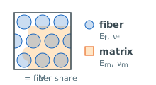
Two phases, one ply
Every model treats the ply as two phases, fiber and matrix, perfectly bonded, with no voids and every fiber running the same way. You give each phase its stiffness on the Fiber and Matrix tabs, and Vf sets how much of the volume is fiber. The matrix is isotropic. The fiber usually is not: a carbon fiber is far stiffer along its axis than across it, so the Fiber tab takes Ef1 and Ef2 separately.
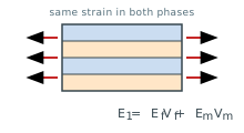
Along the fibers: the rule of mixtures
Pull the ply along the fibers and both phases stretch by the same amount. Each one then carries load in proportion to its stiffness and its share of the volume, so E1 is the volume-weighted average of the fiber and matrix moduli, and ν12 averages the same way. Four of the five models use this rule as it stands. CCA adds a small term for the Poisson mismatch between fiber and matrix.
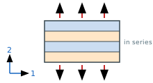
Across the fibers: each model takes its own path
Load the ply across the fibers and the picture changes. The load now passes through fiber and matrix in turn, and the soft matrix takes most of the stretch, so E2 and G12 land much closer to the matrix values. How close depends on how the model idealizes that load path. Rule of Mixtures puts the phases strictly in series, which is the lower bound. Halpin-Tsai adds a fitted reinforcement factor. Chamis and Hopkins-Chamis use a square fiber cell, and CCA an elasticity solution for concentric cylinders.
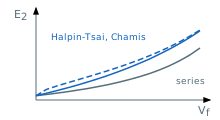
Compare the models, then carry one on
The results table puts the five models side by side at your Vf. They agree on E1 and spread on E2. Switch to the Vf sweep to see that spread across the whole range, and click the chart to set Vf. If you have coupon data, pick the model that matches it. Click its row, then the button under the results, and the laminate calculator opens with that ply.