
From Fiber Volume Fraction to Laminate Stiffness
Fiber and matrix in, quasi-isotropic laminate out. Move Vf and follow it through.
Problem
A [0/45/-45/90]s laminate is made of T300 carbon fiber in an epoxy matrix. How do its in-plane moduli Ex, Ey and Gxy change as the fiber volume fraction goes from 0.3 to 0.7? Work it in two steps: micromechanics from fiber and matrix to the ply, then Classical Lamination Theory from the ply to the laminate.
Materials
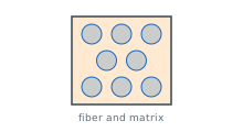
T300 carbon fiber and an epoxy matrix.
Ply
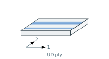
Micromechanics mixes them into one ply at your fiber volume fraction.
Laminate
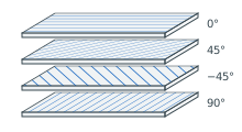
Lamination theory stacks that ply as [0/45/-45/90]s.
Inputs
| Fiber | T300 carbon |
| Ef1 / Ef2 | 230 / 15 GPa |
| Gf12 | 27 GPa |
| νf12 | 0.2 |
| Matrix | Epoxy 3501-6 |
| Em | 4.28 GPa |
| νm | 0.34 |
| Layup | [0/45/-45/90]s, 0.125 mm plies |
These are the presets the free micromechanics calculator opens with. Its default model is the rule of mixtures1: E1 and ν12 mix by volume, E2 and G12 by the inverse rule.
Gm = Em/(2(1 + νm)), since the matrix is isotropic. The laminate moduli then come from the inverse of the A matrix, Ex = 1/(h·a11) and so on1.
Change the fiber volume fraction
Solid lines are the ply, dashed lines the laminate. The dashed vertical line follows the slider.
| At Vf = 0.60, ply | E1 140, E2 7.49, G12 3.67 GPa, ν12 0.256 |
| Laminate | Ex = Ey 52.0, Gxy 19.8 GPa |
In words: from Vf 0.3 to 0.7, ply E1 rises in a straight line from 72.0 to 162 GPa. Ply E2 and G12 stay under 8.56 GPa and curve upward. Laminate Ex goes from 27.6 to 60.8 GPa and Gxy from 10.4 to 23.2 GPa.
Open each step with the slider's Vf:
- Micromechanics calculator, with these fiber and matrix properties
- Ply calculator, for ply thickness and weight at this Vf
- Laminate calculator, with this ply in [0/45/-45/90]s
Results
More fiber stiffens the ply along the fibers almost in proportion. The quasi-isotropic laminate gains nearly as much, because the 0° direction of each ply still carries most of its stiffness. E2 rises only 57% over the same range.
Ply and laminate constants at four fiber volume fractions, moduli in GPa.
| Vf | E1 | E2 | G12 | ν12 | Ex = Ey | Gxy |
|---|---|---|---|---|---|---|
| 0.40 | 94.6 | 5.99 | 2.56 | 0.284 | 35.6 | 13.5 |
| 0.50 | 117 | 6.66 | 3.02 | 0.270 | 43.7 | 16.6 |
| 0.60 | 140 | 7.49 | 3.67 | 0.256 | 52.0 | 19.8 |
| 0.70 | 162 | 8.56 | 4.68 | 0.242 | 60.8 | 23.2 |
Both steps match an independent implementation: the ply constants to the precision it prints, the laminate moduli to six significant figures. Ex equals Ey because the layup is quasi-isotropic in-plane.
What it means
The fiber carries the 0° direction, so E1 tracks Vf directly. Across the fibers the soft matrix sits in series with the fiber, and E2 and G12 stay close to the matrix values until Vf gets high. A quasi-isotropic laminate averages over all directions. Its Ex stays between 37% and 38% of ply E1 across the chart.
The inverse rule of mixtures is a lower bound for E2 and G12. Real plies are usually stiffer across the fibers, and models such as Halpin-Tsai predict more. The micromechanics calculator lists them side by side, so you can see how much the choice moves the laminate. E1 barely depends on the model.
For a real part, measure Vf or get it from the fiber areal weight and cured ply thickness. The fiber volume fraction page shows how.
Related docs:
References
- Jones, R.M., Mechanics of Composite Materials, 2nd Ed., Taylor & Francis, 1999. Section 3.2 (rule of mixtures), Section 4.2 (Classical Lamination Theory).